This is archived from John Norstad's now defunct norstad.org.
Table of Contents
Introduction
The Fallacy of Time Diversification
The Utility Theory Argument
Probability of Shortfall
The Option Pricing Theory Argument
Human Capital
Conclusion
Appendix - A Better Bar Chart Showing Risk Over Time
Introduction
In an otherwise innocent conversation on the Vanguard Diehards forum on the Morningstar web site, I questioned the popular opinion that the risk of investing in volatile assets like stocks decreases as one's time horizon increases. I mentioned that several highly respected Financial Economists believe this opinion to be simply wrong, or at least highly suspect, and that after much study I have come to agree with them. Taylor Larimore asked me to explain. Hence this note.
The following sections are largely independent. Each one presents a single argument. All but the last section present arguments against the popular opinion. The last section presents what I think is the only valid argument supporting the popular opinion.
Past experience tells me that I am unlikely to win any converts with this missive. It's possible, however, that the ideas presented here will make someone think a bit harder about his unexamined assumptions, and will in some small way make him a wiser person. I hope so. In any case, I have wanted to write up my thoughts on this problem for some time now, and I thank Taylor for giving me the little nudge I needed to actually sit down and do it.
If there is one thing I would like people to learn from this paper, it is to disabuse them of the popular notion that stock investing over long periods of time is safe because good and bad returns will somehow "even out over time." Not only is this common opinion false, it is dangerous. There is real risk in stock investing, even over long time horizons. This risk is not necessarily bad, because it is accompanied by the potential for great rewards, but we cannot and should not ignore the risk.
This paper led to a lively debate on Morningstar where the nice Diehards and I exchanged a long sequence of messages on conversations 5266 and 5374. If you find this paper interesting, you might also want to check out those conversations.
The Fallacy of Time Diversification
Portfolio theory teaches that we can decrease the uncertainty of a portfolio without sacrificing expected return by diversifying over a wide range of assets and asset classes. Some people think that this principle can also be used in the time dimension. They argue that if you invest for a long enough time, good and bad returns tend to "even out" or "cancel each other out," and hence time diversifies a portfolio in much the same way that investing in multiple assets and asset classes diversifies a portfolio.
For example, one often hears advice like the following: "At your young age, you have enough time to recover from any dips in the market, so you can safely ignore bonds and go with an all stock retirement portfolio." This kind of statement makes the implicit assumption that given enough time good returns will cancel out any possible bad returns. This is nothing more than a popular version of the supposed "principle" of time diversification. It is usually accepted without question as an obvious fact, made true simply because it is repeated so often, a kind of mean reversion with a vengeance.
In the investing literature, the argument for this principle is often made by observing that as the time horizon increases, the standard deviation of the annualized return decreases. I most frequently see this illustrated as a bar chart displaying a decreasing range of historical minimum to maximum annualized returns over increasing time periods. Some of these charts are so convincing that one is left with the impression that over a very long time horizon investing is a sure thing. After all, look at how tiny those 30 and 40 year bars are on the chart, and how close the minimum and maximum annualized returns are to the average. Give me enough time for all those ups and downs in the market to even out and I can't lose!
While the basic argument that the standard deviations of the annualized returns decrease as the time horizon increases is true, it is also misleading, and it fatally misses the point, because for an investor concerned with the value of his portfolio at the end of a period of time, it is the total return that matters, not the annualized return. Because of the effects of compounding, the standard deviation of the total return actually increases with time horizon. Thus, if we use the traditional measure of uncertainty as the standard deviation of return over the time period in question, uncertainty increases with time.
(The incurious can safely skip the math in this paragraph.) To be precise, in the random walk model, simply compounded rates of return and portfolio ending values are lognormally distributed. Continuously compounded rates of returns are normally distributed. The standard deviation of the annualized continuously compounded returns decreases in proportion to the square root of the time horizon. The standard deviation of the total continuously compounded returns increases in proportion to the square root of the time horizon. Thus, for example, a 16 year investment is 4 times as uncertain as a 1 year investment if we measure "uncertainty" as standard deviation of continuously compounded total return.
As an example, those nice bar charts would look quite different and would certainly leave quite a different impression on the reader if they properly showed minimum and maximum total returns rather than the misleading minimum and maximum annualized returns. As time increases, we'd clearly be able to see that the spread of possible ending values of our portfolio, which is what we care about, gets larger and larger, and hence more and more uncertain. After 30 or 40 years the spreads are quite enormous and clearly show how the uncertainty of investing increases dramatically at very long horizons. Investing over these long periods of time suddenly changes in the reader's mind from a sure thing to a very unsure thing indeed!
For an example of a bar chart which shows a better picture of uncertainty and risk over time, see the Appendix below.
Common variants of this time diversification argument can be found in many popular books and articles on investing, including those by highly respected professionals and even academics. For example, John Bogle used this argument in his otherwise totally excellent February, 1999 speech The Clash of the Cultures in Investing: Complexity vs. Simplicity (see his chart titled "Risk: The Moderation of Compounding 1802-1997," which if it had been properly drawn might well have been titled "Risk: The Exacerbation of Compounding 1802-1997"). Burton Malkiel uses a similar argument and chart in his classic book A Random Walk Down Wall Street (see chapter 14 of the sixth edition). (I deliberately chose two of my all-time favorite authors here to emphasize just how pervasive this fallacy is in the literature.)
The fact that some highly respected, justly admired and otherwise totally worthy professionals use this argument does not make it correct. The argument is in fact just plain wrong - it's a fallacy, pure and simple. When you see it you should dismiss it in the same way that you dismiss urban legends about alligators in sewers and hot stock tips you find on the Internet (you do dismiss those, don't you? :-). It's difficult to do this because the argument is so ubiquitous that it has become an unquestioned assumption in the investment world.
For more details on this fallacy, see the textbook Investments by Bodie, Kane, and Marcus (fourth edition, chapter 8, appendix C), or sections 6.7 and 6.8 of my own paper Random Walks.
The Utility Theory Argument
Robert Merton and Paul Samuelson (both recipients of the Nobel prize in Economic Sciences) use the following argument (among others) to dispute the notion that time necessarily ameliorates risk, and are responsible for much of the mathematics behind the argument. Their argument involves utility theory, a part of Economics which requires a bit of introduction.
Most investors are "risk-averse." For example, a risk-averse investor would refuse to play a "fair game" where he has an equal chance of losing or winning the same amount of money, for an expected return of 0%. Whenever the outcome of an investment is uncertain, a risk-averse investor demands an expected return greater than 0% as a "risk premium" that compensates him for undertaking the risk of the investment. (Actually, such an investor demands an expected return in excess of the risk-free rate, but we'll ignore that detail for the moment.) In general, investors demand higher risk premiums for more volatile investments. One of the fundamental truths of the marketplace is that risk and return always go hand-in-hand in this way. (To be precise, "systematic risk" and "excess return" always go hand-in-hand. Fortunately these are once again details that we don't need to worry about in this paper.)
In Economics the classic way to measure this notion of "risk aversion" is by using "utility functions." A utility function gives us a way to measure an investor's relative preference for different levels of wealth and to measure his willingness to undertake different amounts of risk in the hope of attaining greater wealth. Among other things, formalizing the notion of risk aversion using utility functions makes it possible to develop the mathematics of portfolio optimization. Thus utility theory lies at the heart of and is a prerequisite for modern portfolio theory.
There's a special class of utility functions called the "iso-elastic" functions which characterizes those investors whose relative attitudes towards risk are independent of wealth. For example, suppose you have a current wealth of $10,000 and your preferred asset allocation with your risk tolerance is 50% stocks and 50% bonds for some fixed time horizon. Now suppose your wealth is $100,000 instead of $10,000. Would you change your portfolio's asset allocation for the same time horizon? If you wouldn't, and if you wouldn't change your asset allocation at any other level of wealth either, then you have an iso-elastic utility function (by definition, whether you know it or not). These iso-elastic functions have the property of "constant relative risk aversion."
Note that the definition of these iso-elastic functions is stated in terms of an investor's risk preferences at different levels of wealth, over some fixed time horizon (e.g., 1 year). The property of "constant relative risk aversion" means that the investor's preferred asset allocation (relative exposure to risk) is constant with respect to wealth over this fixed horizon. For the same fixed time horizon, this kind of investor prefers the same asset allocation at all levels of wealth. We aren't ready yet to start talking about other time horizons. We'll get to that later.
While there's no reason to believe that any given investor has or should have iso-elastic utility, it seems reasonable to say that such a hypothetical investor is not pathological. Indeed, constant relative risk aversion is often used as a neutral benchmark against which investor's attitudes towards risk and wealth are measured.
For example, one reasonable investor might be more conservative when he is rich, perhaps because he is concerned about preserving the wealth he has accumulated, whereas when he is poor he takes on more risk, perhaps because he feels he's going to need much more money in the future. This investor has "increasing relative risk aversion."
On the other hand, a different equally reasonable investor might have the opposite attitude. She is more aggessive when she is rich, perhaps because she feels at some point that she already has more than enough money, so she can afford to take on more risk with the excess, whereas when she is poor, she is more concerned about losing the money she needs to live on, so she is more conservative. This investor has "decreasing relative risk aversion."
We can easily imagine more complicated scenarios, where an investor might have increasing relative risk aversion over one range of wealth and decreasing relative risk aversion over some other range.
These attitudes are all reasonable possibilities. All of these investors are risk-averse. They differ only in their degree of risk aversion and their patterns of risk aversion as their wealth increases and decreases. None of the utility functions corresponding to these preferences and patterns are right or wrong or better or worse than the other ones. Everything depends on the individual investor's attitudes. Utility theory does not dictate or judge these attitudes, it just gives us a way to measure them.
In any case, we often think of iso-elastic utility with constant relative risk aversion as a kind of central or neutral position.
Note once again that up to this point in the discussion we have kept the time horizon fixed at some constant value (e.g., 1 year). We have not yet talked about how attitudes towards risk might change with time horizon. All we have talked about so far is how attitudes towards risk might change with wealth over the same fixed time horizon.
Now we're ready for the interesting part of the argument, where we finally make the time horizon a variable. If time necessarily ameliorates risk, one would expect that any rational investor's optimal asset allocation would become more aggressive with longer time horizons. For example, one would certainly expect this to be true for investors with middle-of-the-road iso-elastic utility.
When we do the simple math using calculus and probability theory in the random walk model, however, we get a big surprise. This is not at all what happens. For iso-elastic utility functions, relative attitudes towards risk are also necessarily independent of time horizon. For example, if a 50/50 stock/bond asset allocation is optimal for a 1 year time horizon for an investor with iso-elastic utility, it is also optimal for a 20 year time horizon and all other time horizons!
To summarize, if a rational investor's relative attitudes towards risk are independent of wealth, they are also necessarily independent of time horizon. This is a deep result tying together the three notions of risk, wealth, and time. The result is counter-intuitive to many, but it is nonetheless true. The mathematics is inescapable.
Note once again that we are not arguing that all investors, or even most investors, have iso-elastic utility. The use of iso-elastic utility in this argument simply calls into question the conventional wisdom that time ameliorates risk under all circumstances, regardless of one's attitudes towards risk and wealth. The argument should make people who believe unconditionally that time ameliorates risk to be at least willing to rethink their position.
For more information about utility theory see my paper An Introduction to Utility Theory. For the complete formal proof that investors with iso-elastic utility have the same optimal asset allocation at all time horizons in the random walk model, see my paper An Introduction to Portfolio Theory. Beware: both papers have lots of mathematics. For the almost incomprehensibly complex (but fascinating) math in the general case where the investor is permitted to modify his portfolio continuously through time, see Robert Merton's exquisitely difficult book Continuous Time Finance. (Someday I hope to know enough about all this stuff to actually understand this book. That day is still rather far away, I'm afraid, but it's a goal worth striving towards, and sometimes I actually manage to fool myself into thinking that I'm making some progress.)
Probability of Shortfall
Another argument often found in the popular literature on investing is that as the time horizon increases, the probability of losing money in a risky investment decreases, at least for normal investments with positive expected returns. This is true both when one looks at historical market return data and in the abstract random walk model. (This, by the way, is essentially the argument that Taylor Larimore presented in the Morningstar conversation referred to in the Introduction.) It's even true if we consider not just the probability of losing money, but the probability of making less money than we could in a risk-free investment like US Treasury bonds, provided that our risky investment has an expected return higher than that of T-Bonds.
For example, in the random walk model of the S&P; 500 stock market index in the Appendix below, the probability that a stock investment will earn less than a bank account earning 6% interest is 42% after 1 year. After 40 years this probability decreases to only 10%. Doesn't this prove that risk decreases with time?
The problem with this argument is that it treats all shortfalls equally. A loss of $1000 is treated the same as a loss of $1! This is clearly not fair. For example, if I invest $5000, a loss of $1000, while less likely, is certainly a more devastating loss to me than is a loss of $1, and it should be weighted more heavily in the argument. Similarly, the argument treats all gains equally, which is not fair by the same reasoning.
As a first example, consider a simple puzzle which I hope will make this problem clear. Suppose for the sake of argument that "probability of loss," which is a special case of "probability of shortfall," is a good definition of the "risk" of an investment. Consider two investments A and B which both cost $1000. With A, there's a 50% chance of making $500 and a 50% chance of losing $1. With B, there's a 50% chance of making $1 and a 50% chance of losing $500. A and B have exactly the same probability of loss: 50%. Therefore A and B have exactly the same "risk." What's wrong with this picture?
As a second example, suppose you had the opportunity to make some kind of strange investment which cost $5000 and which had two possible outcomes. In the good case, which has probability 99%, you make $500. In the bad case, which has probability 1%, you lose your entire $5000. Is this a good investment? If not, why not - the probability of loss is only 1%, isn't it? Can't we safely ignore such a small chance of losing money? This investment even has a positive expected rate of return of 8.9%! In this kind of extreme example the problem becomes obvious. This is perhaps not such a great investment after all, at least for some people, because we simply must take into account both the probabilities of the possible outcomes and their magnitudes, not just the probability that we're going to lose money.
To make the problem even worse, suppose you're a starving graduate student with only $5000 to your name, and you need that money to pay your tuition. Is this a good investment for you? Now suppose instead that you're Bill Gates. Would you be willing to risk the loss of an insignificant fraction of your fortune to make a profit of $500 with probability 99%? The situation changes a bit, doesn't it? It seems clear that we also must somehow take into account the investor's current total wealth when we investigate the meaning of "risk" in our example.
As one last mental experiment using this example, how would the situation change if in the bad case you only lost $1000, one fifth of your investment, instead of all of it? The probability of loss is still the same 1%, but it's really a radically different problem, isn't it?
The point of our deliberately extreme pair of examples is that the probability of shortfall measure is much too oversimplified to be a reliable measure of the "risk" of an investment.
Our third example is more realistic. In this example we look at investing in the S&P; 500 stock market index over 1 year and over 3 years.
To begin, we compute that the probability of losing money in the S&P; 500 random walk model is 31% over 1 year but drops to 19% after 3 years. If we use the naive definition of risk as "probability of loss," we would stop thinking about the problem at this point and conclude that the 3 year investment is less risky than the 1 year investment. We hope that at this point in the discussion, however, the reader is convinced that we need to look further.
The probability of losing 20% or more of our money in the S&P; 500 is 5.0% after 1 year. The probability is 6.4% after 3 years. This bad outcome is actually more likely after 3 years than it is after 1 year!
The situation rapidly deteriorates when we start to look at the really bad outcomes, the ones that really scare us. Losing 30% or more of our money is 2.8 times more likely after 3 years than it is after 1 year. Losing 40% or more of our money is 9.7 times more likely after 3 years than it is after 1 year. Losing 50% or more of our money is a whopping 71 times more likely after 3 years than it is after 1 year!
When we start looking at more of the possible outcomes than just the single "lose money" outcome, the risk picture becomes much less clear. It is no longer quite so obvious that the 3 year investment is less risky than the 1 year investment. We start to realize that the situation is more complicated than we had first thought.
Let's take a detour from all this talk about abstract math models for a moment and interject a historical note to go along with our third example. Astute readers might argue at this point that the probabilities of these really bad outcomes, in the 20-50% loss range, are very small, and they would be correct. Isn't it kind of silly to pay all this attention to these low probability possibilities? Can't we safely ignore them? One need only look to the years 1930-1932 to dismiss this argument. Over that 3 year period the S&P; 500 lost 61% of its value. In comparison, US Treasury bills gained 4.5% over the same period. There is no reason to believe that the same thing or even worse can't happen again in the future, perhaps over even longer time periods. It's interesting to note that the S&P; 500 has never had a loss anywhere near as large as 61% in a single year. (The largest one year loss was 43% in 1931.) It took three years of smaller losses to add up to the 61% total loss over 1930-1932. This illustrates the point we made in our example that disastrous losses actually become more likely over longer time horizons.
If you think that 3 years is too short a period of time, and that given more time stock investing must inevitably be a sure bet, consider the 15 years from 1968 through 1982, when after adjusting for inflation the S&P; 500 lost a total of 4.62%. Don't forget that with today's new inflation-protected US bonds, you could easily guarantee an inflation-adjusted return of 25% over 15 years (using a conservative estimate of a 1.5% annualized return in excess of inflation), no matter how bad inflation might get in the future. Are you really prepared to say beyond a shadow of a doubt that a period of high inflation and low stock returns like 1968-1982 can't happen again within your lifetime, or something even worse? Some older people in the US remember this period, which wasn't all that long ago, and they'll tell you that it was a very unpleasant time indeed to be a stock investor. If you'd like another example, consider the near total collapse of the German financial markets between the two world wars, or the recent experience of the Japanese markets, or the markets in other countries during prolonged bad periods in their histories, which in many cases lasted much longer than 15 years. Do you really feel that it's a 100% certainty that something like this couldn't happen here in the US? If we're going to take this notion of "risk" seriously, don't we have to deal with these possibilities, even if they have low probabilities? That in a nutshell is what our argument is all about. It's not just the theory and the abstract math models which teach us that risk is real over long time horizons. History teaches the same lesson.
While we cannot let these disastrous possible outcomes dominate our decision making, and none of the arguments in this paper do so, we also cannot dismiss them just because they're unlikely and they frighten us. Once again, when we think about risk, we have to consider both the magnitudes and the probabilities of all the possible outcomes. This includes the good ones, the bad ones, and the ones in the middle. None of the possible outcomes can be ignored, and none can be permitted to dominate.
Now let's return to our example of the S&P; 500 under-performing a 6% risk-free investment with probability 42% after 1 year but with a probability of only 10% after 40 years. The reason we cannot immediately conclude that the 40 year S&P; 500 investment is less risky than the 1 year investment is that over 40 years the spread of possible outcomes is very wide, and truly disastrous shortfalls of very large magnitudes become more likely, albeit still very unlikely. For sufficiently large possible shortfalls, they actually become much more likely after 40 years than they were after 1 year! We must take these possibilities into account in our assessment of the risk of the 40 year investment. We cannot simply pretend they don't exist or treat them the same as small losses. Similarly, truly enormous gains become more likely, and we must take those into account too. We have to consider all the possibilities.
To solve the problem with using probability of shortfall as a measure of risk, we must at least attach greater negative weights to losses of larger magnitude and greater positive weights to gains of larger magnitude. Then we must somehow take the (probabilistic) average of the weighted possibilities to come up with a fair measure of "risk." How can we do this? This is exactly what utility theory is all about - the assignment of appropriate weights to possible outcomes. Utility theory also addresses the problem of changes in attitudes towards risk as a function of an investor's current wealth.
In the risk-averse universe in which we live, gains and losses of equal magnitude do not just cancel out, so the math isn't trivial. A loss of $x is more of a "bad thing" than a gain of $x is a "good thing." In utility theory this is called "decreasing marginal utility of wealth," and it's equivalent to the notion of "risk aversion." In particular, really disastrous large losses are weighted quite heavily, as they should be. They may have tiny probabilities, but we still need to consider them. For each possible outcome, we need to consider both the probability of the outcome and the weight of the outcome.
When we do the precise calculations using utility theory and integral calculus, the results are inconclusive. As we saw in the previous section, for iso-elastic utility functions with constant relative risk aversion, risk is independent of time, in the sense that the optimal asset allocation is the same at all time horizons. For other kinds of utility functions, risk may increase or decrease with time horizon, depending on the investor.
There is no reason to believe that all investors or even the mythical "typical" or "average" investor has any one particular kind of utility function.
To summarize, simple probability of shortfall is an inadequate measure of risk because it fails to take into account the magnitudes of the possible shortfalls and gains. When we attempt to correct this simple measure of risk by taking the magnitudes into account, we are led to utility theory, which tells us that there is no absolute sense in which we can claim that risk either increases or decreases with time horizon. All it tells us is that it depends on the individual investor, his current wealth, and his risk tolerance patterns as expressed by his particular utility function. For some investors, in this model we can say that risk increases with time. For others, risk decreases with time. For still others, risk is independent of time.
While this may seem inconclusive, and it is, there is one thing that we can conclude: The often-heard probability of shortfall argument in no way proves or even argues convincingly that time ameliorates risk. You should dismiss such arguments whenever you see them, and if you do any reading about investments at all, you will see them frequently. Don't be lulled into a false sense of security by these arguments.
The Option Pricing Theory Argument
Zvi Bodie, a Finance professor at Boston University, came up with an elegant argument that proves that risk actually increases with time horizon, at least for one reasonable definition of "risk." His argument uses the theory of option pricing and the famous Black-Scholes equation. This shouldn't scare the reader, though, because Bodie's argument is really quite simple and easy to understand, and we're going to give a real life example later that doesn't involve any fancy math at all.
Suppose we have a portfolio currently invested in the stock market for some time horizon. One of our alternatives is to sell the entire portfolio and put all of our money into a risk-free zero-coupon US Treasury bond which matures at the same time horizon. (A "zero-coupon" bond pays all of its interest when it matures. This is commonly used as the standard risk-free investment over a fixed time horizon, because all of the payoff occurs at the end of the time period, and the payoff is guaranteed by the US government. This is as close to "risk-free" as we can get in the real world.)
It is reasonable to think of the "risk" of our stock investment being not making as much money as we would with the bond. If we accept this notion of "risk," it then makes sense to measure the magnitude of the risk as being the cost of an insurance policy against a possible shortfall. That is, if someone sells us such a policy, and if at our time horizon we haven't made as much money in the stock market as we would have made with the bond, then the insurer will make up the difference.
This insurance policy is nothing more or less than a European put option on our stock portfolio. The strike price of the option is the payoff of the bond at the end of our time period. The expiration date of the option is the end of our time period. In fact, put options are frequently used in the real world for exactly this kind of "portfolio insurance."
If you plug all the numbers into the Black-Scholes equation for pricing European put and call options, you end up with a very simple equation in which it is clear that the price of the put option increases with time to expiration. In fact, one of the first things students of options learn is the general rule that the price of an option (put or call) increases with time to expiration. It turns out this is even true when we let the strike price increase over time at the risk-free rate. We have taken the price of our put option to be our measure of the magnitude of the risk of our stock investment. Thus, with this model, risk increases with time.
Let's work this argument out in a more personal way in the hope that it will clarify it and perhaps make the reader do some serious thinking about the issue. Suppose for the sake of discussion that you agree with the conventional wisdom that risk decreases with time horizon. In that case, if you were in the business of selling portfolio insurance, would you offer discounts on your policies for longer time horizons? If you really believe in your opinion, then you should be willing to do this, shouldn't you? For example, you should be willing to sell someone an insurance policy against a shortfall after ten years for less money than you'd be willing to sell someone else an otherwise identical policy against a shortfall after one year. After all, according to your beliefs, your risk of having to pay off on the policy is smaller after ten years than it is after one year.
If this is really how you feel, and if you agree with the scenario outlined in the previous paragraph, then you must also feel that the Black-Scholes equation is wrong. Perhaps Black, Scholes, and Merton made some horrible mistake in their derivation of the equation. Not a small mistake either - they must have reversed a sign somewhere! If this is the case, we'd better run over to the Chicago Board Options Exchange and let all those option traders with their Black-Scholes calculators know that they've been doing it wrong all these years. (Maybe they'd get it right if they all held their calculators upside down to read the answers. :-)
We must emphasize that this is not just some arcane theory with no practical application. Option traders buy and sell this kind of portfolio insurance in the form of put options every day in the real life financial markets.
As a concrete example which we'll examine in some detail, let's look at what insurance policies are selling for today, on April 9, 2000. We'll look at CBOE put options on the S&P; 500 stock market index and compare short-term prices for June 2000 options against longer-term prices for December 2001 options.
The S&P; 500 index is currently at 1,516. Current interest rates are about 6%. On June 17, 2000, 2.3 months from now, 1,516 would grow to 1,533 at 6% interest. On December 22, 2001, 20.4 months from now, 1,516 would grow to 1,675 at 6% interest. (If you're wondering where these exact dates come from, options on the CBOE expire on the first Saturday following the third Friday of each month.)
According to today's quotes on the CBOE web site, June 2000 put options on the S&P; 500 with a strike price of 1,533 are selling at about $58. December 2001 put options on the S&P; 500 with a strike price of 1,675 are selling at about $188. (I had to do a bit of mild interpolation to get these numbers, but whatever small errors were introduced do not significantly affect our example.)
To make the example even more concrete, let's suppose you currently have $151,600 invested in Vanguard's S&P; 500 index fund. If you wanted to buy an insurance policy against your fund earning less money than you could in a bank CD or with a US Treasury bill at 6% interest, you could easily call your broker or log on to your online trading account and buy such a policy in the options market. For a 2.3 month time horizon, you would have to pay $5,800 for your policy. For a 20.4 month time horizon, you would have to pay $18,800. (Plus a juicy commission for your broker or online trading company, of course, but we'll ignore that unpleasant detail.)
Thus, right now, professional option traders apparently believe that the risk of the S&P; 500 under-performing a 6% risk-free investment is more than 3 times greater over a 20.4 month horizon than it is over a 2.3 month horizon. This is not some quirk of our example that's only true today or with our specific numbers and dates. In the real life options market this basic phenomenon of portfolio insurance policies costing significantly more for longer time horizons is virtually always true.
In this example, if you believe that the risk of investing in the S&P; 500 decreases with time horizon, and in particular that there's less risk over 20.4 months than there is over 2.3 months, there are only three possibilities:
- You are wrong.
- Professional option traders are wrong.
- There's something wrong with Bodie's simple definition of "risk."
Which is it? It makes you think, doesn't it? Of all the arguments presented so far, I find this one the most convincing.
For the original complete argument see Bodie's paper titled "On the Risk of Stocks in the Long Run" in the Financial Analysts Journal, May-June 1995. You can also find a version of the argument with more of the mathematics than I presented here, plus a graph showing risk increasing over time, in section 6.8 of my paper Random Walks.
Human Capital
The only argument I find valid for the popular opinion that the risk of investing in stocks decreases with time horizon, and in particular the popular opinion that young people should have more aggressive portfolios, involves something called "human capital."
"Human capital" is simply the Economist's fancy term for all the money you will earn at your job for the rest of your working life (discounted to present value using an appropriate discount rate, but we needn't go into those details here.)
The basic argument is that retired people who obtain living expenses from the earnings of their investment portfolios cannot afford as much risk as younger people with long working lives ahead of them and the accompanying regular paychecks.
In this model, the older you get, the less working years you have left, and the smaller your human capital becomes. Thus as you age and get closer to retirement, your investment portfolio should gradually become more conservative.
Note, however, that most retirees do not obtain 100% of their income from investment portfolios. Social security benefits, pensions, and annuities provide steady income streams for many retirees. For our purposes, these guaranteed sources of regular income are no different than the regular income received from a paycheck prior to retirement. Any complete treatment of the issue of adjusting the aggressiveness of a portfolio before and after retirement must take these sources of income into account.
Note also that this argument doesn't work well in some cases. For example, an aerospace engineer whose entire investment portfolio consists of stock in his employer's company is playing a risky game indeed. Similarly, people employed in the investment world would suffer from a high correlation between their human capital and their portfolio, and they might be well-advised to be a bit more conservative than other people of the same age working outside the investment world.
These issues are complicated. Modeling them formally involves a complete life cycle model that takes into account income, consumption, and investment both before and after retirement, and treats human capital and other sources of income as part of the risk aversion computation machinery for determining optimal portfolio asset allocations. I don't pretend to understand all the math yet (it's more of that horribly complicated stuff Merton does), but I hope to some day!
Conclusion
Nearly everyone shares the "obvious" opinion that if you have a longer time horizon, you can afford to and should have a more aggressive investment portfolio than someone with a shorter time horizon. Indeed, it's difficult to visit any web site on investing or read any article or book on investing without being reminded of this "fact" by all sorts of pundits, experts, and professionals, using all kinds of fancy and convincing charts, graphs, statistics, and even (in the case of the web) state of the art interactive Java applets! (For an example of a Java applet, see Time vs. Risk: The Long-Term Case for Stocks [ed -- link to www.smartmoney.com/ac/retirement/investing/index.cfm?story=timerisk hasn't worked for years, maybe even decades] at the SmartMoney web site. It's a great example of the fallacy of time diversification in action.)
On close examination, however, we discover that most of the arguments made in support of this opinion, on those occasions when any argument other than "common sense" is given at all, are either fallacious or at best highly suspect and misleading.
The more we learn about this problem and think about it, the more we come to realize that it's possible that the situation isn't as obvious as we had thought, and that perhaps "common sense" isn't a reliable road to the truth, as is often the case in complex situations which involve making decisions under conditions of uncertainty. In these situations we must build and test models and use mathematics to derive properties of the models. The fact that our mathematics sometimes leads to results which we find counter-intuitive is not sufficient reason to discard the results out of hand. People who have studied a significant amount of math or science will not find it surprising that the truth is often counter-intuitive. Others find this more difficult to accept, but accept it they must if they wish to take these problems seriously.
We have seen at least one compelling argument (Bodie's option pricing theory argument) that the opposite of the commonly held belief is true: If we assume an entirely reasonable definition of the notion of "risk," the risk of investing in volatile assets like stocks actually increases with time horizon!
The only argument supporting the conventional wisdom that survives close examination is the one relying on human capital. Younger people with secure long-term employment prospects may in some circumstances have good reason to be somewhat more aggressive than older people or those with less secure employment prospects.
In any case, the most commonly heard arguments which rely on the fallacy of time diversification or which use probability of shortfall as a risk measure are clearly flawed and should be ignored whenever they are encountered, which is, alas, all too frequently.
Appendix - A Better Bar Chart Showing Risk Over Time
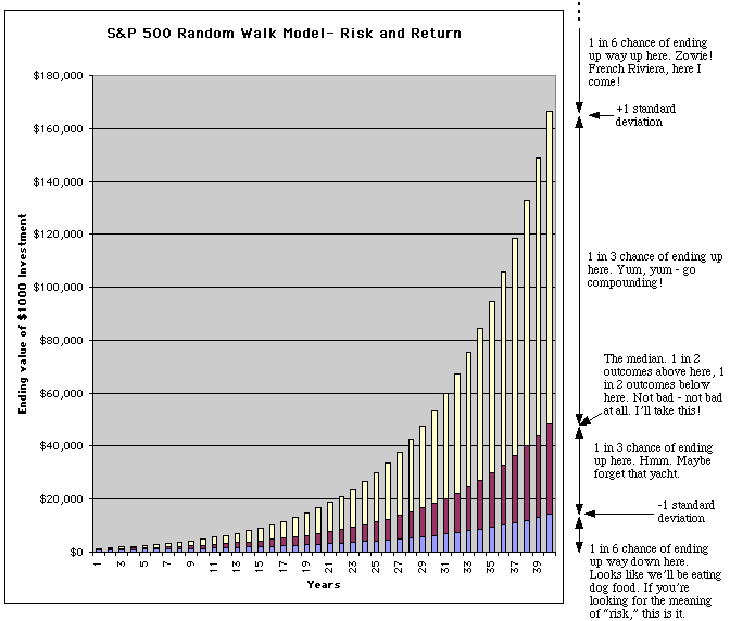
This chart shows the growth of a $1000 investment in a random walk model of the S&P; 500 stock market index over time horizons ranging from 1 to 40 years. It pretty much speaks for itself, I hope - that was the intention, anyway.
The chart clearly shows the dramatic increasing uncertainty of an S&P; 500 stock investment as time horizon increases. For example, at 40 years, the chart gives only a 2 in 3 chance that the ending value will be somewhere between $14,000 and $166,000. This is an enormous range of possible outcomes, and there's a significant 1 in 3 chance that the actual ending value will be below or above the range! You can't get much more uncertain than this.
As long as we're talking about risk, let's consider a really bad case. If instead of investing our $1000 in the S&P; 500, we put it in a bank earning 6% interest, after 40 years we'd have $10,286. This is 1.26 standard deviations below the median ending value of the S&P; 500 investment. The probability of ending up below this point is 10%. In other words, even over a very long 40 year time horizon, we still have about a 1 in 10 chance of ending up with less money than if we had put it in the bank!
Look at the median curve - the top of the purple rectangles, and follow it with your eye as time increases. You see the typical geometric growth you get with the magic of compounding. Imagine the chart if all we drew was that curve, so we were illustrating only the median growth curve without showing the other possible outcomes and their ranges. It would paint quite a different picture, wouldn't it? When you're doing financial planning, it's extremely important to look at both return and risk.
There's one problem with this chart. It involves a phenomenon called "reversion to mean." Some (but not all) academics and other experts believe that over long periods of time financial markets which have done better than usual in the past tend to do worse than usual in the future, and vice-versa. The effect of this phenomenon on the pure random walk model we've used to draw the chart is to decrease somewhat the standard deviations at longer time horizons. The net result is that the dramatic widening of the spread of possible outcomes shown in the chart is not as pronounced. The +1 standard deviation ending values (the tops of the bars) come down quite a bit, and the -1 standard deviation ending values come up a little bit. The phenomenon is not, however, anywhere near so pronounced as to actually make the +1 and -1 standard deviation curves get closer together over time. The basic conclusion that the uncertainty of the ending values increases with time does not change.
For those who might be interested in how I created the chart, here's the details:
I first got historical S&P; 500 total return data from 1926 through 1994 from Table 2.4 in the book Finance by Zvi Bodie and Robert Merton.
I typed the data into Microsoft Excel, converted all the simply compounded yearly returns into continuous compounding (by taking the natural logarithm of one plus each simply compounded return), and then computed the mean and the standard deviation. I got the following pair of numbers "mu" and "sigma":
mu = 9.7070% = Average annual continuously compounded return. This corresponds to an average annual simply compounded return of 12.30% (the arithmetic mean) and an average annualized simply compounded return of 10.19% (the geometric mean).
sigma = 19.4756% = The standard deviation of the annual continuously compounded returns.
(The steps up to this point were actually done a long time ago for other projects.)
I then used Excel to draw the bar chart. At t years, the -1 standard deviation, median, and +1 standard deviation ending values were computed by the following formulas:
-1 s.d. ending value = 1000*exp(mu*t - sigma*sqrt(t))
median ending value = 1000*exp(mu*t)
+1 s.d. ending value = 1000*exp(mu*t + sigma*sqrt(t))
I then copied the chart from Excel to the drawing module in the AppleWorks program and used AppleWorks to annotate it and save it as a GIF file that I could use in this web page.