This is a pseudo-transcript for a talk on branch prediction given at Two Sigma on 8/22/2017 to kick off "localhost", a talk series organized by RC.
How many of you use branches in your code? Could you please raise your hand if you use if statements or pattern matching?
Most of the audience raises their hands
I won’t ask you to raise your hands for this next part, but my guess is that if I asked, how many of you feel like you have a good understanding of what your CPU does when it executes a branch and what the performance implications are, and how many of you feel like you could understand a modern paper on branch prediction, fewer people would raise their hands.
The purpose of this talk is to explain how and why CPUs do “branch prediction” and then explain enough about classic branch prediction algorithms that you could read a modern paper on branch prediction and basically know what’s going on.
Before we talk about branch prediction, let’s talk about why CPUs do branch prediction. To do that, we’ll need to know a bit about how CPUs work.
For the purposes of this talk, you can think of your computer as a CPU plus some memory. The instructions live in memory and the CPU executes a sequence of instructions from memory, where instructions are things like “add two numbers”, “move a chunk of data from memory to the processor”. Normally, after executing one instruction, the CPU will execute the instruction that’s at the next sequential address. However, there are instructions called “branches” that let you change the address next instruction comes from.
Here’s an abstract diagram of a CPU executing some instructions. The x-axis is time and the y-axis distinguishes different instructions.
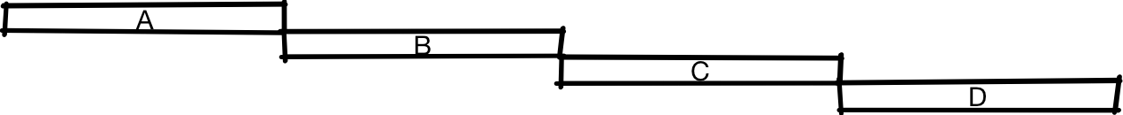
Here, we execute instruction A, followed by instruction B, followed by instruction C, followed by instruction D.
One way you might design a CPU is to have the CPU do all of the work for one instruction, then move on to the next instruction, do all of the work for the next instruction, and so on. There’s nothing wrong with this; a lot of older CPUs did this, and some modern very low-cost CPUs still do this. But if you want to make a faster CPU, you might make a CPU that works like an assembly line. That is, you break the CPU up into two parts, so that half the CPU can do the “front half” of the work for an instruction while half the CPU works on the “back half” of the work for an instruction, like an assembly line. This is typically called a pipelined CPU.
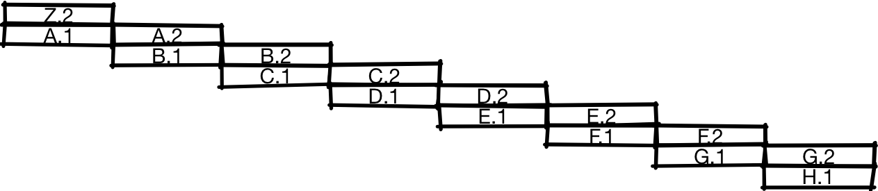
If you do this, the execution might look something like the above. After the first half of instruction A is complete, the CPU can work on the second half of instruction A while the first half of instruction B runs. And when the second half of A finishes, the CPU can start on both the second half of B and the first half of C. In this diagram, you can see that the pipelined CPU can execute twice as many instructions per unit time as the unpipelined CPU above.
There’s no reason that a CPU can only be broken up into two parts. We could break the CPU into three parts, and get a 3x speedup, or four parts and get a 4x speedup. This isn’t strictly true, and we generally get less than a 3x speedup for a three-stage pipeline or 4x speedup for a 4-stage pipeline because there’s overhead in breaking the CPU up into more parts and having a deeper pipeline.
One source of overhead is how branches are handled. One of the first things the CPU has to do for an instruction is to get the instruction; to do that, it has to know where the instruction is. For example, consider the following code:
if (x == 0) {
  // Do stuff
} else {
  // Do other stuff (things)
}
  // Whatever happens later
This might turn into assembly that looks something like
branch_if_not_equal x, 0, else_label
// Do stuff
goto end_label
else_label:
// Do things
end_label:
// whatever happens later
In this example, we compare x to 0. if_not_equal, then we branch to else_label and execute the code in the else block. If that comparison fails (i.e., if x is 0), we fall through, execute the code in the if block, and then jump to end_label in order to avoid executing the code in else block.
The particular sequence of instructions that’s problematic for pipelining is
branch_if_not_equal x, 0, else_label
???
The CPU doesn’t know if this is going to be
branch_if_not_equal x, 0, else_label
// Do stuff
or
branch_if_not_equal x, 0, else_label
// Do things
until the branch has finished (or nearly finished) executing. Since one of the first things the CPU needs to do for an instruction is to get the instruction from memory, and we don’t know which instruction ??? is going to be, we can’t even start on ??? until the previous instruction is nearly finished.
Earlier, when we said that we’d get a 3x speedup for a 3-stage pipeline or a 20x speedup for a 20-stage pipeline, that assumed that you could start a new instruction every cycle, but in this case the two instructions are nearly serialized.
One way around this problem is to use branch prediction. When a branch shows up, the CPU will guess if the branch was taken or not taken.
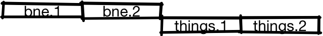
In this case, the CPU predicts that the branch won’t be taken and starts executing the first half of stuff while it’s executing the second half of the branch. If the prediction is correct, the CPU will execute the second half of stuff and can start another instruction while it’s executing the second half of stuff, like we saw in the first pipeline diagram.
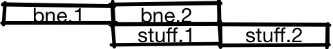
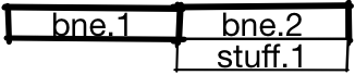
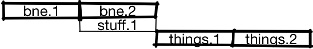
If the prediction is wrong, when the branch finishes executing, the CPU will throw away the result from stuff.1 and start executing the correct instructions instead of the wrong instructions. Since we would’ve stalled the processor and not executed any instructions if we didn’t have branch prediction, we’re no worse off than we would’ve been had we not made a prediction (at least at the level of detail we’re looking at).
What’s the performance impact of doing this? To make an estimate, we’ll need a performance model and a workload. For the purposes of this talk, our cartoon model of a CPU will be a pipelined CPU where non-branches take an average of one instruction per clock, unpredicted or mispredicted branches take 20 cycles, and correctly predicted branches take one cycle.
If we look at the most commonly used benchmark of “workstation” integer workloads, SPECint, the composition is maybe 20% branches, and 80% other operations. Without branch prediction, we then expect the “average” instruction to take branch_pct * 1 + non_branch_pct * 20 = 0.2 * 20 + 0.8 * 1 = 4 + 0.8 = 4.8 cycles. With perfect, 100% accurate, branch prediction, we’d expect the average instruction to take 0.8 * 1 + 0.2 * 1 = 1 cycle, a 4.8x speedup! Another way to look at it is that if we have a pipeline with a 20-cycle branch misprediction penalty, we have nearly a 5x overhead from our ideal pipelining speedup just from branches alone.
Let’s see what we can do about this. We’ll start with the most naive things someone might do and work our way up to something better.
Predict taken
Instead of predicting randomly, we could look at all branches in the execution of all programs. If we do this, we’ll see that taken and not not-taken branches aren’t exactly balanced -- there are substantially more taken branches than not-taken branches. One reason for this is that loop branches are often taken.
If we predict that every branch is taken, we might get 70% accuracy, which means we’ll pay the the misprediction cost for 30% of branches, making the cost of of an average instruction (0.8 + 0.7 * 0.2) * 1 + 0.3 * 0.2 * 20 = 0.94 + 1.2. = 2.14. If we compare always predicting taken to no prediction and perfect prediction, always predicting taken gets a large fraction of the benefit of perfect prediction despite being a very simple algorithm.

Backwards taken forwards not taken (BTFNT)
Predicting branches as taken works well for loops, but not so great for all branches. If we look at whether or not branches are taken based on whether or not the branch is forward (skips over code) or backwards (goes back to previous code), we can see that backwards branches are taken more often than forward branches, so we could try a predictor which predicts that backward branches are taken and forward branches aren’t taken (BTFNT). If we implement this scheme in hardware, compiler writers will conspire with us to arrange code such that branches the compiler thinks will be taken will be backwards branches and branches the compiler thinks won’t be taken will be forward branches.
If we do this, we might get something like 80% prediction accuracy, making our cost function (0.8 + 0.8 * 0.2) * 1 + 0.2 * 0.2 * 20 = 0.96 + 0.8 = 1.76 cycles per instruction.

Used by
- PPC 601(1993): also uses compiler generated branch hints
- PPC 603
One-bit
So far, we’ve look at schemes that don’t store any state, i.e., schemes where the prediction ignores the program’s execution history. These are called static branch prediction schemes in the literature. These schemes have the advantage of being simple but they have the disadvantage of being bad at predicting branches whose behavior change over time. If you want an example of a branch whose behavior changes over time, you might imagine some code like
if (flag) {
  // things
  }
Over the course of the program, we might have one phase of the program where the flag is set and the branch is taken and another phase of the program where flag isn’t set and the branch isn’t taken. There’s no way for a static scheme to make good predictions for a branch like that, so let’s consider dynamic branch prediction schemes, where the prediction can change based on the program history.
One of the simplest things we might do is to make a prediction based on the last result of the branch, i.e., we predict taken if the branch was taken last time and we predict not taken if the branch wasn’t taken last time.
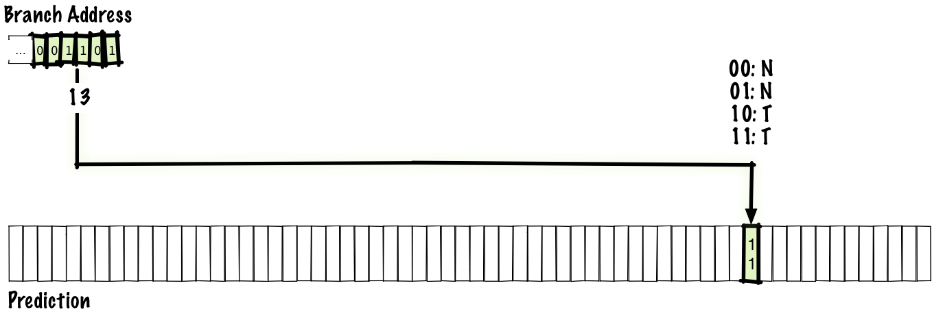
Since having one bit for every possible branch is too many bits to feasibly store, we’ll keep a table of some number of branches we’ve seen and their last results. For this talk, let’s store not taken as 0 and taken as 1.
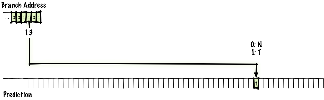
In this case, just to make things fit on a diagram, we have a 64-entry table, which mean that we can index into the table with 6 bits, so we index into the table with the low 6 bits of the branch address. After we execute a branch, we update the entry in the prediction table (highlighted below) and the next time the branch is executed again, we index into the same entry and use the updated value for the prediction.
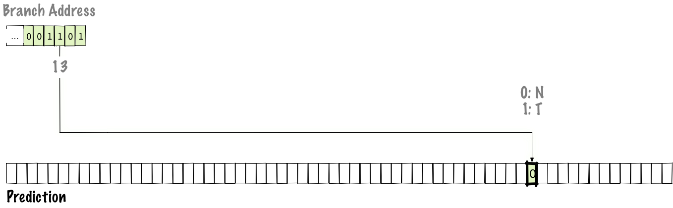
It’s possible that we’ll observe aliasing and two branches in two different locations will map to the same location. This isn’t ideal, but there’s a tradeoff between table speed & cost vs. size that effectively limits the size of the table.
If we use a one-bit scheme, we might get 85% accuracy, a cost of (0.8 + 0.85 * 0.2) * 1 + 0.15 * 0.2 * 20 = 0.97 + 0.6 = 1.57 cycles per instruction.

Used by
- DEC EV4 (1992)
- MIPS R8000 (1994)
A one-bit scheme works fine for patterns like TTTTTTTT… or NNNNNNN… but will have a misprediction for a stream of branches that’s mostly taken but has one branch that’s not taken, ...TTTNTTT... This can be fixed by adding second bit for each address and implementing a saturating counter. Let’s arbitrarily say that we count down when a branch is not taken and count up when it’s taken. If we look at the binary values, we’ll then end up with:
00: predict Not
01: predict Not
10: predict Taken
11: predict Taken
The “saturating” part of saturating counter means that if we count down from 00, instead of underflowing, we stay at 00, and similar for counting up from 11 staying at 11. This scheme is identical to the one-bit scheme, except that each entry in the prediction table is two bits instead of one bit.
Compared to a one-bit scheme, a two-bit scheme can have half as many entries at the same size/cost (if we only consider the cost of storage and ignore the cost of the logic for the saturating counter), but even so, for most reasonable table sizes a two-bit scheme provides better accuracy.
Despite being simple, this works quite well, and we might expect to see something like 90% accuracy for a two bit predictor, which gives us a cost of 1.38 cycles per instruction.

One natural thing to do would be to generalize the scheme to an n-bit saturating counter, but it turns out that adding more bits has a relatively small effect on accuracy. We haven’t really discussed the cost of the branch predictor, but going from 2 bits to 3 bits per branch increases the table size by 1.5x for little gain, which makes it not worth the cost in most cases. The simplest and most common things that we won’t predict well with a two-bit scheme are patterns like NTNTNTNTNT... or NNTNNTNNT…, but going to n-bits won’t let us predict those patterns well either!
Used by
- LLNL S-1 (1977)
- CDC Cyber? (early 80s)
- Burroughs B4900 (1982): state stored in instruction stream; hardware would over-write instruction to update branch state
- Intel Pentium (1993)
- PPC 604 (1994)
- DEC EV45 (1993)
- DEC EV5 (1995)
- PA 8000 (1996): actually a 3-bit shift register with majority vote
If we think about code like
for (int i = 0; i < 3; ++i) {
  // code here.
  }
That code will produce a pattern of branches like TTTNTTTNTTTN....
If we know the last three executions of the branch, we should be able to predict the next execution of the branch:
TTT:N
TTN:T
TNT:T
NTT:T
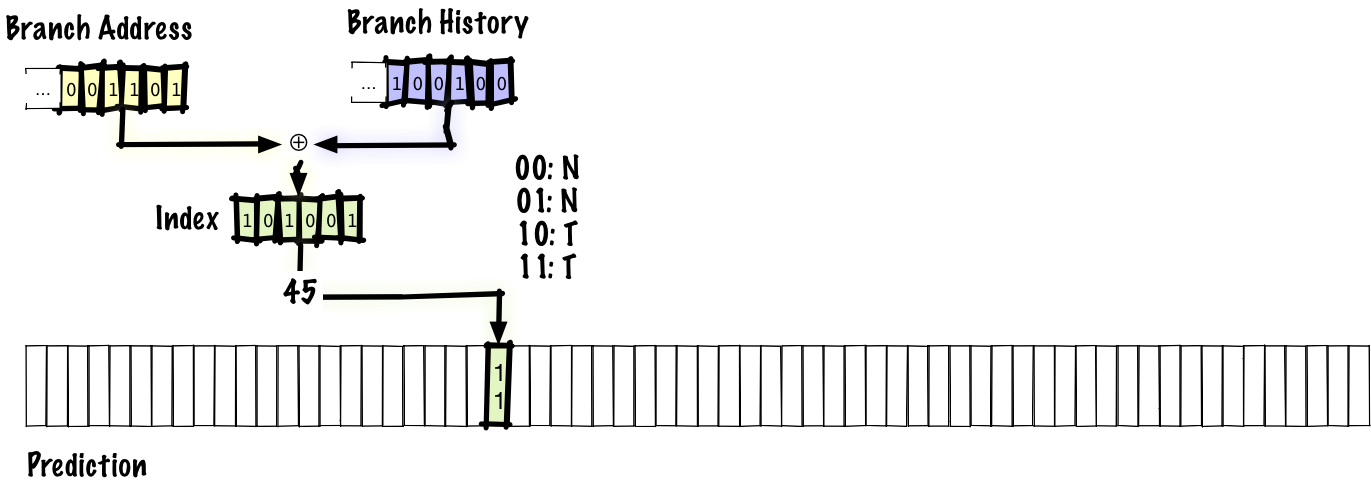
The previous schemes we’ve considered use the branch address to index into a table that tells us if the branch is, according to recent history, more likely to be taken or not taken. That tells us which direction the branch is biased towards, but it can’t tell us that we’re in the middle of a repetitive pattern. To fix that, we’ll store the history of the most recent branches as well as a table of predictions.
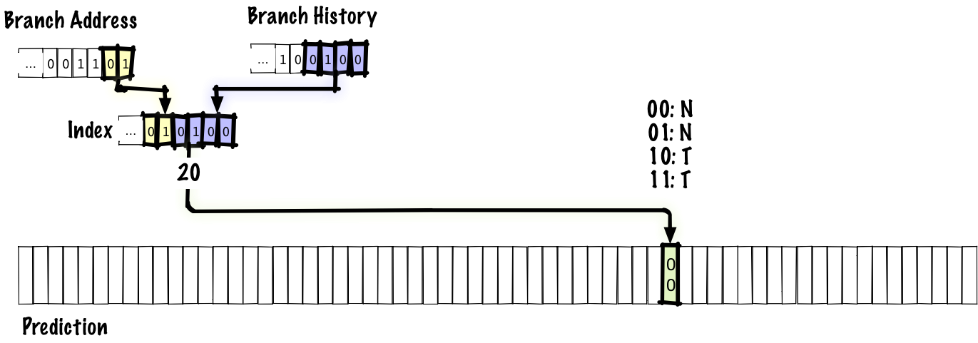
In this example, we concatenate 4 bits of branch history together with 2 bits of branch address to index into the prediction table. As before, the prediction comes from a 2-bit saturating counter. We don’t want to only use the branch history to index into our prediction table since, if we did that, any two branches with the same history would alias to the same table entry. In a real predictor, we’d probably have a larger table and use more bits of branch address, but in order to fit the table on a slide, we have an index that’s only 6 bits long.
Below, we’ll see what gets updated when we execute a branch.
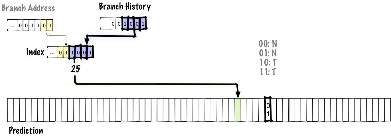
The bolded parts are the parts that were updated. In this diagram, we shift new bits of branch history in from right to left, updating the branch history. Because the branch history is updated, the low bits of the index into the prediction table are updated, so the next time we take the same branch again, we’ll use a different entry in the table to make the prediction, unlike in previous schemes where the index is fixed by the branch address. The old entry’s value is updated so that the next time we take the same branch again with the same branch history, we’ll have the updated prediction.
Since the history in this scheme is global, this will correctly predict patterns like NTNTNTNT… in inner loops, but may not always correct make predictions for higher-level branches because the history is global and will be contaminated with information from other branches. However, the tradeoff here is that keeping a global history is cheaper than keeping a table of local histories. Additionally, using a global history lets us correctly predict correlated branches. For example, we might have something like:
if x > 0:
  x -= 1
if y > 0:
  y -= 1
if x * y > 0:
  foo()
If either the first branch or the next branch isn’t taken, then the third branch definitely will not be taken.
With this scheme, we might get 93% accuracy, giving us 1.27 cycles per instruction.

Used by
- Pentium MMX (1996): 4-bit global branch history
As mentioned above, an issue with the global history scheme is that the branch history for local branches that could be predicted cleanly gets contaminated by other branches.
One way to get good local predictions is to keep separate branch histories for separate branches.
Instead of keeping a single global history, we keep a table of local histories, index by the branch address. This scheme is identical to the global scheme we just looked at, except that we keep multiple branch histories. One way to think about this is that having global history is a special case of local history, where the number of histories we keep track of is 1.
With this scheme, we might get something like 94% accuracy, which gives us a cost of 1.23 cycles per instruction.

Used by
gshare
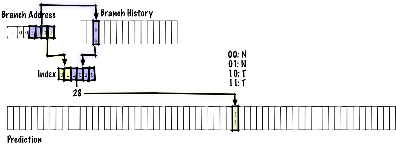
One tradeoff a global two-level scheme has to make is that, for a prediction table of a fixed size, bits must be dedicated to either the branch history or the branch address. We’d like to give more bits to the branch history because that allows correlations across greater “distance” as well as tracking more complicated patterns and we’d like to give more bits to the branch address to avoid interference between unrelated branches.
We can try to get the best of both worlds by hashing both the branch history and the branch address instead of concatenating them. One of the simplest reasonable things one might do, and the first proposed mechanism was to xor them together. This two-level adaptive scheme, where we xorthe bits together is called gshare.
With this scheme, we might see something like 94% accuracy. That’s the accuracy we got from the local scheme we just looked at, but gshare avoids having to keep a large table of local histories; getting the same accuracy while having to track less state is a significant improvement.
Used by
One reason for branch mispredictions is interference between different branches that alias to the same location. There are many ways to reduce interference between branches that alias to the same predictor table entry. In fact, the reason this talk only runs into schemes invented in the 90s is because a wide variety of interference-reducing schemes were proposed and there are too many to cover in half an hour.
We’ll look at one scheme which might give you an idea of what an interference-reducing scheme could look like, the “agree” predictor. When two branch-history pairs collide, the predictions either match or they don’t. If they match, we’ll call that neutral interference and if they don’t, we’ll call that negative interference. The idea is that most branches tend to be strongly biased (that is, if we use two-bit entries in the predictor table, we expect that, without interference, most entries will be 00 or 11 most of the time, not 01 or 10). For each branch in the program, we’ll store one bit, which we call the “bias”. The table of predictions will, instead of storing the absolute branch predictions, store whether or not the prediction matches or does not match the bias.
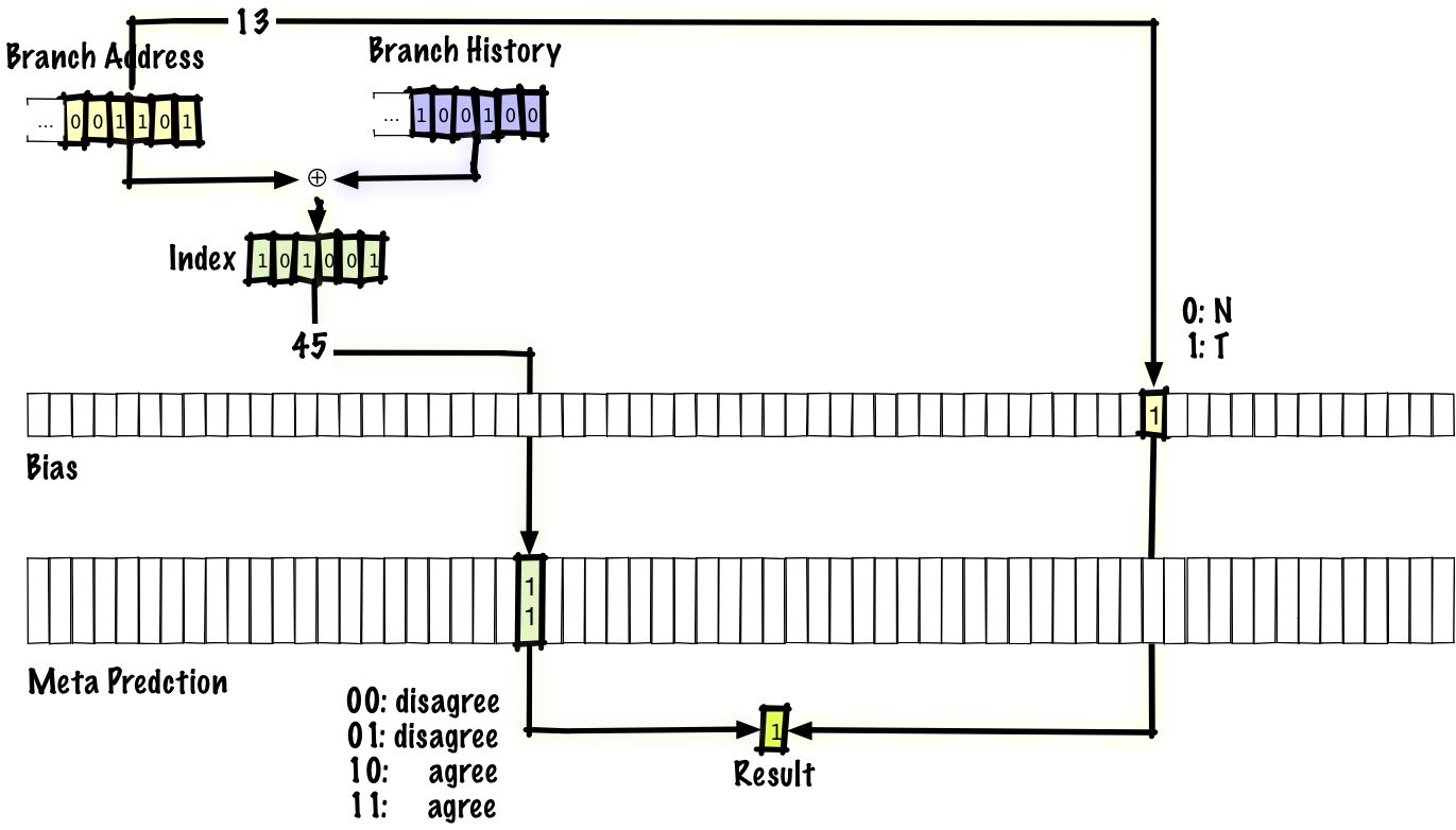
If we look at how this works, the predictor is identical to a gshare predictor, except that we make the changes mentioned above -- the prediction is agree/disagree instead of taken/not-taken and we have a bias bit that’s indexed by the branch address, which gives us something to agree or disagree with. In the original paper, they propose using the first thing you see as the bias and other people have proposed using profile-guided optimization (basically running the program and feeding the data back to the compiler) to determine the bias.
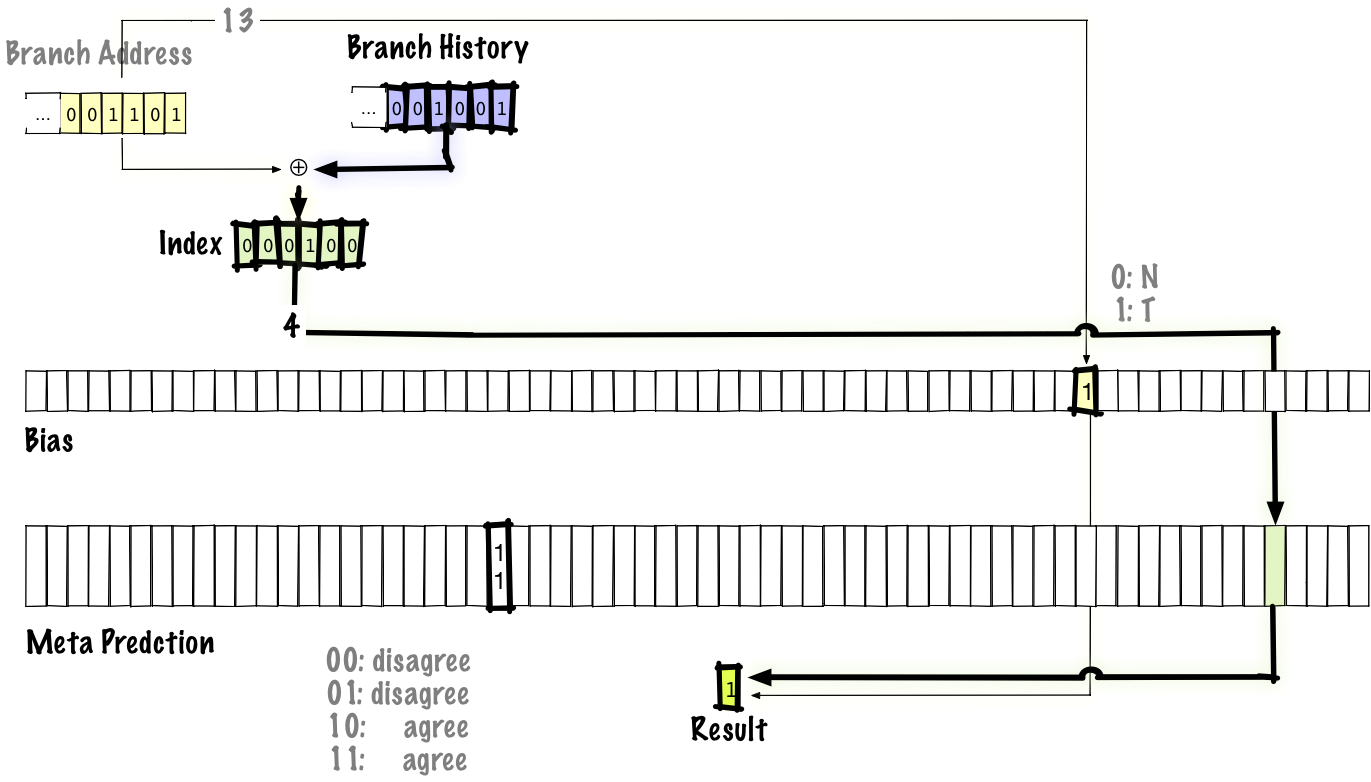
Note that, when we execute a branch and then later come back around to the same branch, we’ll use the same bias bit because the bias is indexed by the branch address, but we’ll use a different predictor table entry because that’s indexed by both the branch address and the branch history.
If it seems weird that this would do anything, let’s look at a concrete example. Say we have two branches, branch A which is taken with 90% probability and branch B which is taken with 10% probability. If those two branches alias and we assume the probabilities that each branch is taken are independent, the probability that they disagree and negatively interfere is P(A taken) * P(B not taken) + P(A not taken) + P(B taken) = (0.9 * 0.9) + (0.1 * 0.1) = 0.82.
If we use the agree scheme, we can re-do the calculation above, but the probability that the two branches disagree and negatively interfere is P(A agree) * P(B disagree) + P(A disagree) * P(B agree) = P(A taken) * P(B taken) + P(A not taken) * P(B taken) = (0.9 * 0.1) + (0.1 * 0.9) = 0.18. Another way to look at it is, to have destructive interference, one of the branches must disagree with its bias. By definition, if we’ve correctly determined the bias, this cannot be likely to happen.
With this scheme, we might get something like 95% accuracy, giving us 1.19 cycles per instruction.

Used by
As we’ve seen, local predictors can predict some kinds of branches well (e.g., inner loops) and global predictors can predict some kinds of branches well (e.g., some correlated branches). One way to try to get the best of both worlds is to have both predictors, then have a meta predictor that predicts if the local or the global predictor should be used. A simple way to do this is to have the meta-predictor use the same scheme as the two-bit predictor above, except that instead of predicting taken or not taken it predicts local predictor or global predictor
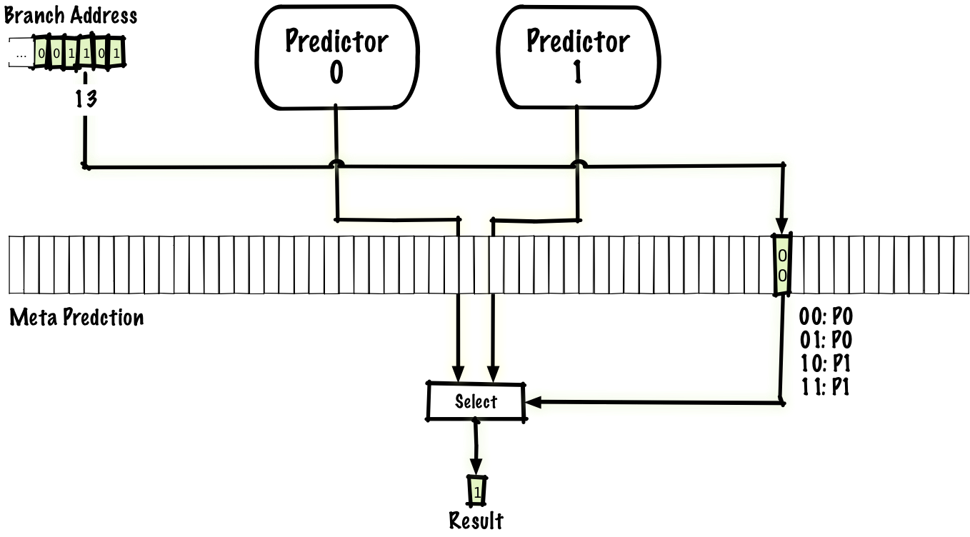
Just as there are many possible interference-reducing schemes, of which the agree predictor, above is one, there are many possible hybrid schemes. We could use any two predictors, not just a local and global predictor, and we could even use more than two predictors.
If we use a local and global predictor, we might get something like 96% accuracy, giving us 1.15 cycles per instruction.

Used by
- DEC EV6 (1998): combination of local (1k entries, 10 history bits, 3 bit counter) & global (4k entries, 12 history bits, 2 bit counter) predictors
- IBM POWER4 (2001): local (16k entries) & gshare (16k entries, 11 history bits, xor with branch address, 16k selector table)
- IBM POWER5 (2004): combination of bimodal (not covered) and two-level adaptive
- IBM POWER7 (2010)
Not covered
There are a lot of things we didn’t cover in this talk! As you might expect, the set of material that we didn’t cover is much larger than what we did cover. I’ll briefly describe a few things we didn’t cover, with references, so you can look them up if you’re interested in learning more.
One major thing we didn’t talk about is how to predict the branch target. Note that this needs to be done even for some unconditional branches (that is, branches that don’t need directional prediction because they’re always taken), since (some) unconditional branches have unknown branch targets.
Branch target prediction is expensive enough that some early CPUs had a branch prediction policy of “always predict not taken” because a branch target isn’t necessary when you predict the branch won’t be taken! Always predicting not taken has poor accuracy, but it’s still better than making no prediction at all.
Among the interference reducing predictors we didn’t discuss are bi-mode, gskew, and YAGS. Very briefly, bi-mode is somewhat like agree in that it tries to seperate out branches based on direction, but the mechanism used in bi-mode is that we keep multiple predictor tables and a third predictor based on the branch address is used to predict which predictor table gets use for the particular combination of branch and branch history. Bi-mode appears to be more successful than agree in that it's seen wider use. With gskew, we keep at least three predictor tables and use a different hash to index into each table. The idea is that, even if two branches alias, those two branches will only alias in one of the tables, so we can use a vote and the result from the other two tables will override the potentially bad result from the aliasing table. I don't know how to describe YAGS very briefly :-).
Because we didn't take about speed (as in latency), a prediction strategy we didn't talk about is to have a small/fast predictor that can be overridden by a slower and more accurate predictor when the slower predictor computes its result.
Some modern CPUs have completely different branch predictors; AMD Zen (2017) and AMD Bulldozer (2011) chips appear to use perceptron based branch predictors. Perceptrons are single-layer neural nets.
It’s been argued that Intel Haswell (2013) uses a variant of a TAGE predictor. TAGE stands for TAgged GEometric history length predictor. If we look at the predictors we’ve covered and look at actual executions of programs to see which branches we’re not predicting correctly, one major class of branches are branches that need a lot of history -- a significant number of branches need tens or hundreds of bits of history and some even need more than a thousand bits of branch history. If we have a single predictor or even a hybrid predictor that combines a few different predictors, it’s counterproductive to keep a thousand bits of history because that will make predictions worse for the branches which need a relatively small amount of history (especially relative to the cost), which is most branches. One of the ideas in the TAGE predictor is that, by keeping a geometric series of history lengths, each branch can use the appropriate history. That explains the GE. The TA part is that branches are tagged, which is a mechanism we don’t discuss that the predictor uses to track which branches should use which set of history.
Modern CPUs often have specialized predictors, e.g., a loop predictor can accurately predict loop branches in cases where a generalized branch predictor couldn’t reasonably store enough history to make perfect predictions for every iteration of the loop.
We didn’t talk at all about the tradeoff between using up more space and getting better predictions. Not only does changing the size of the table change the performance of a predictor, it also changes which predictors are better relative to each other.
We also didn’t talk at all about how different workloads affect different branch predictors. Predictor performance varies not only based on table size but also based on which particular program is run.
We’ve also talked about branch misprediction cost as if it’s a fixed thing, but it is not, and for that matter, the cost of non-branch instructions also varies widely between different workloads.
I tried to avoid introducing non-self-explanatory terminology when possible, so if you read the literature, terminology will be somewhat different.
Conclusion
We’ve looked at a variety of classic branch predictors and very briefly discussed a couple of newer predictors. Some of the classic predictors we discussed are still used in CPUs today, and if this were an hour long talk instead of a half-hour long talk, we could have discussed state-of-the-art predictors. I think that a lot of people have an idea that CPUs are mysterious and hard to understand, but I think that CPUs are actually easier to understand than software. I might be biased because I used to work on CPUs, but I think that this is not a result of my bias but something fundamental.
If you think about the complexity of software, the main limiting factor on complexity is your imagination. If you can imagine something in enough detail that you can write it down, you can make it. Of course there are cases where that’s not the limiting factor and there’s something more practical (e.g., the performance of large scale applications), but I think that most of us spend most of our time writing software where the limiting factor is the ability to create and manage complexity.
Hardware is quite different from this in that there are forces that push back against complexity. Every chunk of hardware you implement costs money, so you want to implement as little hardware as possible. Additionally, performance matters for most hardware (whether that’s absolute performance or performance per dollar or per watt or per other cost), and adding complexity makes hardware slower, which limits performance. Today, you can buy an off-the-shelf CPU for $300 which can be overclocked to 5 GHz. At 5 GHz, one unit of work is one-fifth of one nanosecond. For reference, light travels roughly one foot in one nanosecond. Another limiting factor is that people get pretty upset when CPUs don’t work perfectly all of the time. Although CPUs do have bugs, the rate of bugs is much lower than in almost all software, i.e., the standard to which they’re verified/tested is much higher. Adding complexity makes things harder to test and verify. Because CPUs are held to a higher correctness standard than most software, adding complexity creates a much higher test/verification burden on CPUs, which makes adding a similar amount of complexity much more expensive in hardware than in software, even ignoring the other factors we discussed.
A side effect of these factors that push back against chip complexity is that, for any particular “high-level” general purpose CPU feature, it is generally conceptually simple enough that it can be described in a half-hour or hour-long talk. CPUs are simpler than many programmers think! BTW, I say “high-level” to rule out things like how transistors and circuit design, which can require a fair amount of low-level (physics or solid-state) background to understand.
CPU internals series
Thanks to Leah Hanson, Hari Angepat, and Nick Bergson-Shilcock for reviewing practice versions of the talk and to Fred Clausen Jr for finding a typo in this post. Apologies for the somewhat slapdash state of this post -- I wrote it quickly so that people who attended the talk could refer to the “transcript ” soon afterwards and look up references, but this means that there are probably more than the usual number of errors and that the organization isn’t as nice as it would be for a normal blog post. In particular, things that were explained using a series of animations in the talk are not explained in the same level of detail and on skimming this, I notice that there’s less explanation of what sorts of branches each predictor doesn’t handle well, and hence less motivation for each predictor. I may try to go back and add more motivation, but I’m unlikely to restructure the post completely and generate a new set of graphics that better convey concepts when there are a couple of still graphics next to text. Thanks to Julien Vivenot, Ralph Corderoy, Vaibhav Sagar, Mindy Preston, Stefan Kanthak, and Uri Shaked for catching typos in this hastily written post.