su3su2u1 physics tumblr archive

These are archived from the now defunct su3su2u1 tumblr.

A Roundabout Approach to Quantum Mechanics

This will be the first post in what I hope will be a series that outlines some ideas from quantum mechanics. I will try to keep it light, and not overly math filled- which means I’m not really teaching you physics. I’m teaching you some flavor of the physics. I originally wrote here “you can’t expect to make ice cream just having tasted it,” but I think a better description might be “you can’t expect to make ice cream just having heard someone describe what it tastes like.” AND PLEASE, PLEASE PLEASE ask questions. I’m used to instant feedback on my (attempts at) teaching, so if readers aren’t getting anything out of this, I want to stop or change or something.

Now, unfortunately I can’t start with quantum mechanics without talking about classical physics first. Most people think they know classical mechanics, having learned it on their mother’s knee, but there are so,so many ways to formulate classical physics, and most physics majors don’t see some really important ones (in particular Hamiltonian and Lagrangian mechanics) until after quantum mechanics. This is silly, but at the same time university is only 4 years. I can’t possibly teach you all of these huge topics, but I will need to rely on a few properties of particle and of light. And unlike intro Newtonian mechanics, I want to focus on paths. Instead of asking something like “a particle starts here with some velocity, where does it go?” I want to focus on “a particle starts here, and ends there. What path did it take?”

So today we start with light, and a topic I rather love. Back in the day, before “nerd-sniping” several generations of mathematicians, Fermat was laying down a beautiful formulation of optics-

Light always takes the path of least time

I hear an objection “isn’t that just straight lines?” We have to combine this insight with the notion that light travels at different speeds in different materials. For instance, we know light slows down in water by a factor of about 1.3.

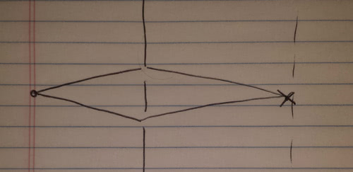
So lets look at a practical problem, you see a fish swimming in water (I apologize in advance for these diagrams):

I drew the (hard to see) dotted straight line between your eye and the fish.

But that isn’t what the light does- there is a path that saves the light some time. The light travels faster in air than in water, so it can travel further in the air, and take a shorter route in the water to the fish.

This is a more realistic path for the light- it bends when it hits the water- it does this in order to take paths of least time between points in the water and points in the air. Exercise for the mathematical reader- you can work this out quantitatively and derive Snell’s law (the law of refraction) just from the principle of least time.

And one more realistic example: Lenses. How do they work?

So that bit in the middle is the lens and we are looking at light paths that leave 1 and travel to 2 (or visa versa, I guess).

The lens is thickest in the middle, so the dotted line gets slowed the most. Path b is longer, but it spends less time in the lens- that means with careful attention to the shape of the lens we can make the time of path b equal to the time of the dotted path.

Path a is the longest path, and just barely touches the lens, so is barely slowed at all, so it too can be made to take the same time as the dotted path (and path b).

So if we design our lens carefully, all of the shortest-time paths that touch the lens end up focused back to one spot.

So thats the principle of least time for light. When I get around to posting on this again we’ll talk about particles.

Now, these sort of posts take some effort, so PLEASE PLEASE PLEASE tell me if you got something out of this.

Edit: And if you didn’t get anything out of this, because its confusing, ask questions. Lots of questions, any questions you like.

More classical physics of paths

So after some thought, these posts will probably be structured by first discussing light, and then turning to matter, topic by topic. It might not be the best structure, but its at least giving me something to organize my thoughts around.

As in all physics posts, please ask questions. I don’t know my audience very well here, so any feedback is appreciated. Also, there is something of an uncertainty principle between clarity and accuracy. I can be really clear or really accurate, but never both. I’m hoping to walk the middle line here.

Last time, I mentioned that geometric optics can be formulated by the simple principle that light takes the path of least time. This is a bit different than many of the physics theories you are used to- generally questions are phrased along the lines of “Alice throws a football from position x, with velocity v, where does Bob need to be to catch the football.” i.e. we start with an initial position and velocity. Path based questions are usually “a particle starts at position x_i,t_i and ends at position x_f,t_f, what path did it take?”

For classical non-relativistic mechanics, the path based formulation is fairly simple, we construct a quantity called the “Lagrangian” which is defined by subtracting potential energy from kinetic energy (KE - PE). Recall that kinetic energy is 1/2 mv^2, where m is the mass of the particle and v is the velocity, and potential energy depends on the problem. If we add up the Lagrangian at every instant along a path we get a quantity called the action (S is the usual symbol for action, for some reason) and particles take the path of least action. If you know calculus, we can put this as

[S = \int KE-PE dt ]

The action has units of energy*time, which will be important in a later post.

Believe it or not, all of Newton’s laws are all contained in this minimization principle. For instance, consider a particle moving with no outside influences (no potential energy). Such a particle has to minimize its v^2 over the path it takes.

Any movement away from the straight line will cause an increase in the length of the path, so the particle will have to travel faster, on average, to arrive at its destination. We want to minimize v^2, so we can deduce right away the particle will take a straight line path.

But what about its speed? Should a particle move very slowly to decrease v^2 as it travels, and then “step on the gas” near the end? Or travel at a constant speed? Its easy to show that minimum action is the constant speed path (give it a try!). This gives us back Newton’s first law.

You can also consider the case of a ball thrown straight up into the air. What path should it take? Now we have potential energy mgh (where h is the height, and g is a gravitational constant). But remember, we subtract the potential energy in the action- so the particle can lower its action by climbing higher.

Along the path of least action in a gravitational field, the particle will move slowly at high h to spend more time at low-action, and will speed up as h decreases (it needs to have an average velocity large enough to get to its destination on time). If you know calculus of variations, you can calculate the required relationship, and you’ll find you get back exactly the Newtonian relationship (acceleration of the particle = g).

Why bother with this formulation? It makes a lot of problems easier. Sometimes specifying all the forces is tricky (imagine a bead sliding on a metal hoop. The hoop constrains the bead to move along the circular hoop, so the forces are just whatever happens to be required to keep the bead from leaving the hoop. But the energy can be written very easily if we use the right coordinates). And with certain symmetries its a lot more elegant (a topic I’ll leave for another post).

So to wrap up both posts- light takes the path of least time, particles take the path of least action. (One way to think about this is that light has a Lagrangian that is constant. This means that the only way to lower the action is to find the path that takes the least time). This is the take away points I need for later- in classical physics particles take the path of least action.

I feel like this is a lot more confusing than previous posts because its hard to calculate concrete examples. Please ask questions if you have them.

Semi classical light

As always math will not render properly on tumblr dash, but will on the blog. This post contains the crux of this whole series of posts, so its really important to try to understand this argument.

Recall from the first post I wrote that one particularly elegant formulation of geometric optics is Fermat’s principle:

light takes the path of least time

But, says a young experimentalist (pun very much intended!), look what happens when I shine light through two slits, I get a pattern like this:

Light must be a wave.

"Wait, wait, wait!" I can hear you saying. Why does this two slit thing mean that light is a wave?

Let us talk about the key feature of waves- when waves come together they can combine in different ways:

TODO: broken link.

So when a physicists want to represent waves, we need to take into account not just the height of the wave, but also the phase of the wave. The wave can be at “full hump” or “full trough” or anywhere in between.

The technique we use is called “phasors” (not to be confused with phasers). We represent waves as little arrows, spinning around in a circle:

TODO: broken link.

The ;length of the arrow A is called the amplitude and represents the height of the wave. The angle, (\theta) represents the phase of the wave. (The mathematical sophisticates among us will recognize these as complex numbers of the form (Ae^{i\theta}) With these arrows, we can capture all the add/subtract/partially-add features of waves:

TODO: broken link.

So how do we use this to explain the double slit experiment? First, we assume all the light that leaves the same source has the same amplitude. And the light has a characteristic period, T. It takes T seconds for the light to go from “full trough” back to “full trough” again.

In our phasor diagram, this means we can represent the phase of our light after t seconds as:

[\theta = \frac{2\pi t}{T} ]

Note, we are taking the angle here in radians. 2 pi is a full circle. That way when t = T, we’ve gone a full circle.

We also know that light travels at speed c (c being the “speed of light,” after all). So as light travels a path of length L, the time it traveled is easily calculated as (\frac{L}{c}).

Now, lets look at some possible paths:

The light moves from the dot on the left, through the two slits, and arrives at the point X. Now, for the point X at the center of the screen, both paths will have equal lengths. This means the waves arrive with no difference in phase, and they add together. We expect a bright spot at the center of the screen (and we do get one).

Now, lets look at points further up the screen:

As we move away from the center, the paths have different lengths, and we get a phase difference in the arriving light:

[\theta_1 - \theta_2= \frac{2\pi }{cT} \left(L_1 - L_2\right) ]

So what happens? As we move up the wall, the length distance gets bigger and the phase difference increases. Every time the phase difference is a multiple of pi we get cancellation, and a dark spot. Every time its a multiple of 2 pi, we get a bright spot. This is exactly Young’s results.

But wait a minute, I can hear a bright student piping up (we’ll call him Feynman, but it would be more appropriate to call him Huygens in this case). Feynman says “What if there were 3 slits?”

Well, then we’d have to add up the phasors for 3 different slits. Its more algebra, but when they all line up, its a bright spot, when they all cancel its a dark spot,etc. We could even have places where two cancel out, and one doesn’t.

"But, what if I made a 4th hole?" We add up four phasors. "A 5th? "We add up 5 phasors.

"What if I drilled infinite holes? Then the screen wouldn’t exist anymore! Shouldn’t we recover geometric optics then?"

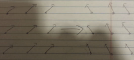
Ah! Very clever! But we DO recover geometric optics. Think about what happens if we add up infinitely many paths. We are essentially adding up infinitely many random phasors of the same amplitude:

So we expect all these random paths to cancel out.

But there is a huge exception.

Those random angles are because when we grab an arbitrary path, the time light takes on that path is random.

But what happens near a minimum? If we parameterize our random paths, near the minimum the graph of time-of-travel vs parameter looks like this:

The graph gets flat near the minimum, so all those little Xs have roughly the same phase, which means all those phasors will add together. So the minimum path gets strongly reinforced, and all the other paths cancel out.

So now we have one rule for light:

To calculate how light moves forward in time, we add up the associated phasors for light traveling every possible path.

BUT, when we have many, many paths we can make an approximation. With many, many paths the only one that doesn’t cancel out, the only one that matters, is the path of minimum time.

Semi-classical particles

Recall from the previous post that we had improved our understanding of light. Light we suggested, was a wave which means

Light takes all possible paths between two points, and the phase of the light depends on the time along the path light takes.

Further, this means:

In situations where there are many, many paths the contributions of almost all the paths cancel out. Only the path of least time contributes to the result.

The astute reader can see where we are going. We already learned that classical particles take the path of least action, so we might guess at a new rule:

Particles take all possible paths between two points, and the phase of the particle depends on the action along the path the particle takes.

Recall from the previous post that the way we formalized this is that the phase of light could be calculated with the formula

[\theta = \frac{2\pi}{T} t]

We would like to make a similar formula for particles, but instead of time it must depend on the action, but will we do for the particle equivalent of the “period?” The simplest guess we might take is a constant. Lets call the constant h, planck’s constant (because thats what it is). It has to have the same units of action, which are energy*time.

[\theta = \frac{2\pi}{h} * S]

Its pretty common in physics to use a slightly different constant (\hbar = \frac{h}{2\pi} ) because it shows up so often.

[\theta = \frac{S}{\hbar}]

So we have this theory- maybe particles are really waves! We’ll just run a particle through a double slit and we’ll see a pattern just like the light!

So we set up our double slit experiment, throw a particle at the screen, and blip. We pick up one point on the other side. Huh? I thought we’d get a wave. So we do the experiment over and over again, and this results

So we do get the pattern we expected, but only built up over time. What do we make of this?

Well, one things seems obvious- the outcome of a large number of experiments fits our prediction very well. So we can interpret the result of our rule as a probability instead of a traditional fully determined prediction. But probabilities have to be positive, so we’ll say the probability is proportional to the square of our amplitude.

So lets rephrase our rule:

To predict the probability that a particle will arrive at a point x at time t, we take a phasor for every possible path the particle can take, with a phase depending on the action along the path, and we add them all up. Squaring the amplitude gives us the probability.

Now, believe it or not, this rule is exactly equivalent to the Schroedinger equation that some of us know and love, and pretty much everything you’ll find in an intro quantum book. Its just a different formulation. But you’ll note that I called it “semi-classical” in the title- thats because undergraduate quantum doesn’t really cover fully quantum systems, but thats a discussion for a later post.

If you are familiar with Yudkowsky’s sequence on quantum mechanics or with an intro textbook, you might be used to thinking of quantum mechancis as blobs of amplitude in configuration space changing with time. In this formulation, our amplitudes are associated with paths through spacetime.

When next I feel like writing again, we’ll talk a bit about how weird this path rule really is, and maybe some advantages to thinking in paths.

Basic special relativity

LNo calculus or light required, special relativity using only algebra. Note- I’m basically typing up some lecture notes here, so this is mostly a sketch.

This derivation is based on key principle that I believe Galileo first formulated-

The laws of physics are the same in any inertial frame OR there is no way to detect absolute motion. Like all relativity derivations, this is going to involve a thought experiment. In our experiment we have a train that moves from one of train platform to the other. At the same time a toy airplane also flies from one of the platform to the other (originally, I had made a Planes,Trains and Automobiles joke here, but kids these days didn’t get the reference… ::sigh::)

There are two events, event 1- everything starts at the left side of the platform. Event 2- everything arrives at the right side of the platform. The entire time the train is moving with a constant velocity v from the platform’s perspective (symmetry tells us this also means that the platform is moving with velocity v from the train’s perspective.)

We’ll look at these two events from two different perspectives- the perspective of the platform and the perspective of the train. The goal is to figure out a set of equations that let us relate quantities between the different perspectives.

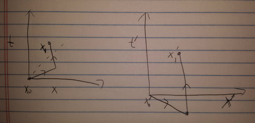
HERE COMES A SHITTY DIAGRAM

The dot is the toy plane, the box is the train. L is the length of the platform from its own perspective. l is the length of the train from it’s own perspective. T is the time it takes the train to cross the platform from the platform’s perspective. And t is the time the platform takes to cross the train from the train’s perspective.

From the platform’s perspective, it’s easy to see the train has length l’ = L - vT. And the toy plane has speed w = L/T.

From the train’s perspective, the platform has length L’ = l + vt and the toy plane has speed u = l/t

So to summarize

Observer | Time passed between events | Length of Train | Speed of Plane

Platform | T | l’ = L-vT | w = L/T

Train | t |L’ = l+vt | u/t

Now, we again exploit symmetry and our Galilean principle. By symmetry,

l’/l = L’/L = R

Now, by the Galilean principle, R as a function can only depend on v. If it didn’t we could detect absolute motion. We might want to just assume R is 1, but we wouldn’t be very careful if we did.

So what we do is this- we want to write a formula for w in terms of u and v and R (which depends only on v). This will tell us how to relate a velocity in the train’s frame to a velocity in the plane’s frame.

I’ll skip the algebra, but you can use the relations above to work this out for yourself

w = (u+v)/(1+(1-R)u/v) = f(u,v)

Here I just used f to name the function there.

I WILL EDIT MORE IN, POSTING NOW SO I DON’T LOSE THIS TYPED UP STUFF.

More Special Relativity and Paths

This won’t make much sense if you haven’t read my last post on relativity. Math won’t render on tumblr dash, instead go to the blog.

Last time, we worked out formulas for length contraction (and I asked you to work out a formula for time dilation). But what would generally be useful is a formula generally relating events between the different frames of reference. Our thought experiment had two events-

event 1, the back end of the train, the back end of the platform, and the toy are all at the same place.

event 2- the front of the train, the front end of the platform, and the toy are all at the same place.

From the toy’s frame of reference, these events occur at the same place, so we only have a difference between the two events. We’ll call that difference (\Delta\tau) . We’ll always use this to mean “the time between events that occur at the same position” (only in one frame will events occur in the same place), and it’s called proper time.

Now, the toy train sees the platform moves with speed -w, and the length of the platform is RL. So this relationship is just time = distance/speed.

[\Delta\tau^2 = R^2L^2/w^2 = (1-\frac{w^2}{c^2})L^2/w^2 ]

Now, we can manipulate the right hand side by noting that from the platform’s perspective, L^2/w^2 is the time between the two events, and those two events are separated by a distance L. We’ll call the time between events in the platforms frame of reference (\Delta t) and the distance between the events L, we’ll call generally (\Delta x).

[\Delta\tau^2 = (1-\frac{w^2}{c^2})L^2/w^2 = (\Delta t^2 - \Delta x^2/c^2) ]

Note that the speed w has dropped out of the final version of the equation- this would be true for any frame, since proper time is unique (every frame has a different time measurement, but only one measures the proper time), we have a frame independent measurement.

Now, lets relate this back to the idea of paths that I’ve discussed previously. One advantage of the path approach to mechanics is that if we can create a special relativity invariant action then the mechanics we get is also invariant. So one way we might consider to do this is by looking at proper time- (remember S is the action). Note the negative sign- without it there is no minimum only a maximum.

[ S \propto -\int d\tau = -C\int d\tau ]

Now C has to have units of energy for the action to have the right units.

Now, some sketchy physics math

[ S = -C\int \sqrt(dt^2 - dx^2/c^2) = -C\int dt \sqrt(1-\frac{dx^2}{dt^2}/c^2) ]

[S = -C\int dt \sqrt(1-v^2/c^2) ]

So one last step is to note that the approximation we can make for \sqrt(1-v^2/c^2), if v is much smaller than c which is (1-1/2v^2/c^2)

So all together, for small v

[S = C\int dt (\frac{v^2}{2c^2} - 1)]

So if we pick the constant C to be mc^2, then we get

[S = \int dt (1/2 mv^2 - mc^2)]

We recognize the first term as just the kinetic energy we had before! The second term is just a constant and so won’t effect where the minimum is. This gives us a new understanding of our path rule for particles- particles take the path of maximum proper time (it’s this understanding of mechanics that translates most easily to general relativity)

Special relativity and free will

Imagine right now, while you are debating whether or not to post something on tumblr, some aliens in the andromeda galaxy are sitting around a conference table discussing andromeda stuff.

So what is the “space time distance” between you right now (deciding what to tumblrize) and those aliens?

Well, the distance between andromeda and us is something like 2.5 million light years. So thats a “space time distance” tau (using our formula from last time) of 2.5 million years. So far, so good:

Now, imagine an alien, running late to the andromeda meeting, is running in. He is running at maybe 1 meter/second. We know that for him lengths will contract and time will dilate. So for him, time on earth is actually later- using

(\Delta \tau^2 = \Delta t^2 - \Delta x^2/ c^2)

and using our formula for length contraction, we can calculate that according to our runner in andromeda the current time on Earth is about 9 days later then today.

So simultaneous to the committee sitting around on andromeda, you are just now deciding what to tumblrize. According to the runner, it’s 9 days later and you’ve already posted whatever you are thinking about + dozens of other things.

So how much free will do you really have about what you post? (This argument is originally due to Rietdijk and Putnam).

We are doing Taylor series in calculus and it's really boring. What would you add from physics?

First, sorry I didn’t get to this for so long.

Anyway, there is a phenomenon in physics where almost everything is modeled as a spring (simple harmonic motion is everywhere!). You can see this in discussion of resonances. Wave motion can be understood as springs coupled together,etc, and lots of system exhibit waves- when you speak the tiny air perurbations travel out like waves, same as throwing a pebble in a pond, or wiggling a jump rope. These are all very different systems, so why the hell do we see such similar behavior?

Why would this be? Well, think of a system in equilibrium, and nudging it a tiny bit away from equilibrium. If the equilibrium is at some parameter a, and we nudge it a tiny bit away from equilibrium (so x-a = epsilon)

[E(x-a)]

Now, we can Taylor expand- but we note that in equiilibrium the energy is at a minimum, so the linear term in the Taylor expansion is 0

[E(\epsilon)= E(a) + \frac{d^2E}{dx^2}1/2 \epsilon^2 + … ]

Now, constants in potential energy don’t matter, and so the first important term is a squared potential energy, which is a spring.

So Taylor series-> everything is a spring.

Why field theory?

So far, we’ve learned in earlier posts in my quantum category that

Classical theories can be described in terms of paths with rules where particles take the path of “least action.”
We can turn a classical theory into a quantum one by having the particle take every path, with the phase from each path given by the action along the path (divided by hbar).

We’ve also learned that we can make a classical theory comply with special relativity by picking a relativistic action (in particle, an action proportional to the “proper time.”)

So one obvious thing to try to make a special relativistic quantum theory would be to start with a special relativistic action and do the sum over paths we use for the classical theory.

You can do this- and it almost works! If you do the mathematical transition from our original, non-relativistic paths to standard, textbook quantum you’d find that you get the Schroedinger equation (or if you were more sophisticated you could get something called the Pauli equation that no one talks about, but is basically the Schroedinger equation + the fact that electrons have spin).

If you try to do it from a relativistic action, you would get an equation called the Klein-Gordon equation (or if you were more sophisticated you could get the Dirac equation). Unfortunately, this runs into trouble- there can be weird negative probabilities, and general weirdness to the solutions.

So we have done something wrong- and the answer is that making the action special relativistic invariant isn’t enough.

Let’s look at some paths:

So the dotted line in this picture represents the light cone- how fast light traveling away from the point will travel. All of the paths end up inside the light cone, but some of the paths go outside of it. This leads to really strange situations, lets look at one outside the light cone path from two frames of reference:

So what we see is that a normal path in the first frame (on the left) looks really strange in the second- because the order of events for events outside the lightcone isn’t fixed, some frame of references see the path as moving back in time.

So immediately we see the problem. When we switched to the relativistic theory we weren’t including all the paths- to really include all the paths we need to include paths that also (apparently) move back in time. This is very strange! Notice that if we run time forward the X’ observer sees ,at some points along the path two particles (one moving back in time, one moving forward).

Feynman’s genius was to demonstrate that we can think of these particles moving backward in time as anti-particles moving forward in time. So the x’ observer

So really our path set looks like

Notice that not only do we have paths connecting the two points, but we have totally unrelated loops that start and end at the same points- these paths are possible now!

So to calculate a probability, we can’t just look at the paths that connect paths connecting points x_o and x_1! There can be weird loopy paths that never touch x_o and x_1 that still matter! From Feynman’s persepctive, particle and anti particle pairs can form, travel awhile and annihilate later.

So as a book keeping device we introduce a field- at every point in space it has a value. To calculate the action of the field we can’t just look at the paths- instead we have to sum up the values of the fields (and some derivatives) at every point in space.

So our old action was a sum of the action over just times (S is the action, L is the lagrangian)

[S = \int dt L ]

Our new action has to be a sum over space and time.

[S = \int dt d^x l ]

So now our Lagrangian is a lagrangian density.

And we can’t just restrict ourselves to paths- we have to add up every possible configuration of the field.

So that’s why we need field theory to combine relativity with quantum mechanics. Next time some implications

Field theory implications

So the first thing is that if we take the Feynman interpretation, our field theory doesn’t have a fixed particle number- depending on the weird loops in a configuration it could have an almost arbitrary number of particles. So one way to phrase the problem with not including backwards paths is that we need to allow the particle number to fluctuate.

Also, I know some of you are thinking “what are these fields?” Well- that’s not so strange. Think of the electromagnetic fields. If you have no charges around, what are the solutions to the electromagnetic field? They are just light waves. Remember this post? Remember that certain special paths were the most important for the sum over all paths? Similarly, certain field configurations are the most important for the sum over configurations. Those are the solutions to the classical field theory.

So if we start with EM field theory, with no charges, then the most important solutions are photons (the light waves). So we can outline levels of approximation

Sum over all configurations -> (semi classical) photons that travel all paths -> (fully classical) particles that travel just the classical path.

Similarly, with any particle

Sum over all configurations -> (semi classical) particles that travel all paths -> (fully classical) particles that travel just the classical path.

This is why most quantum mechanics classes really only cover wave mechanics and don’t ever get fully quantum mechanical.

Planck length/time

Answering somervta's question. What is the significance of Planck units.

Let’s start with an easier one where we have some intuition- let’s analyze the simple hydrogen atom (the go-to quantum mechanics problem). But instead of doing physics, lets just do dimensional analysis- how big do we expect hydrogen energies to be?

Let’s start with something simpler- what sort of distances do we expect a hydrogen atom to have? How big should it’s radius be?

Well, first- what physics is involved? I model the hydrogen atom as an electron moving in an electric field, and I expect I’ll need quantum mechanics, so I’ll need hbar (planck’s constant), e, the charge of the electron, coulomb’s constant (call it k), and the mass of the electron. Can I turn these into a length?

Let’s give it a try- k*e^2 is an energy times a length. hbar is an energy * a time, so if we divide we can get hbar/(k*e^2) which has units of time/length. Multiply in by another hbar, and we get hbar^2/(k*e^2), which has units of mass * length. So divide by the mass of the electron, and we get a quantity hbar^2/(m*k*e^2).

This has units of length, so we might guess that the important length scale for the hydrogen atom is our quantity (this has a value of about 53 picometers, which is about the right scale for atomic hyrdogen).

We could also estimate the energy of the hydrogen atom by noting that

Energy ~ k*e^2/r and use our scale for r.

Energy ~ m*k^2*e^4/(hbar^2) ~27 eV.

This is about twice as large as the actual ground state, but its definitely the right order of magnitude.

Now what Planck noticed is that if you ask “what are the length scales of quantum gravity?” You end up with the constants G, c, and hbar. Turns out, you can make a length scale out of that (sqrt (hbar*G/c^3) ) So just like with hydrogen, we expect that gives us a characteristic length for where quantum effects might start to matter for gravity (or gravity effects might matter for quantum mechanics).

The planck energy and planck mass, then, are similarly characteristic mass and energy scales.

It’s sort of “how small do my lengths have to be before quantum gravity might matter?” But it’s just a guess, really. Planck energy is the energy you’d need to probe that sort of length scale (higher energies probe smaller lengths),etc.

Does that answer your question?

In the standard model, what are the fundamental "beables" (things that exist) and what are kinds of properties do they have (that is, not "how much mass do they have" but "they have mass")?

So this one is pretty tough, because I don’t think we know for sure exactly what the “beables” are (assuming you are using beable like Bell’s term).

The issue is that field theory is formulated in terms of potentials- the fields that enter into the action are the electromagnetic potential, not the electromagnetic field. In classical electromagnetic theory, we might say the electromagnetic field is a beable (Bell’s example), but the potential is not.

But in field theory we calculate everything in terms of potentials- and we consider certain states of the potential to be “photons.”

At the electron level, we have a field configuration that is more general than the wavefunction - different configurations represent different combinations of wavefunctions (one configuration might represent a certain 3 particle wavefunction, another might represent a single particle wavefunction,etc).

In Bohm type theories, the beables are the actual particle positions, and we could do something like that for field theory- assume the fields are just book keeping devices. This runs into problems though, because field configurations that don’t look much like particles are possible, and can have an impact on your theory. So you want to give some reality to the fields.

Another issue is that the field configurations themselves aren’t unique- symmetries relate different field configurations so that very different configurations imply the same physical state.

A lot of this goes back to the fact that we don’t have a realistic axiomatic field theory yet.

But for concreteness sake, assume the fields are “real,” then you have fermion fields, which have a spin of 1/2, an electro-weak charge, a strong charge, and a coupling to the higgs field. These represent right or left handed electrons,muons,neutrinos,etc.

You have gauge-fields (strong field, electro-weak field), these represent your force carrying boson (photons, W,Z bosons, gluons).

And you have a Higgs field, which has a coupling to the electroweak field, and it has the property of being non-zero everywhere in space, and that constant value is called its vacuum expectation value.

What's the straight dope on dark matter candidates?

So, first off there are two types of potential dark matter. Hot dark matter, and cold dark matter. One obvious form of dark matter would be neutrinos- they only interact weakly and we know they exist! So this seems very obvious and promising until you work it out. Because neutrinos are so light (near massless), most of them will be traveling at very near the speed of light. This is “hot” dark matter and it doesn’t have the right properties.

So what we really want is cold dark matter. I think astronomers have some ideas for normal baryonic dark matter (brown dwarfs or something). I don’t know as much about those.

Particle physicists instead like to talk about what we call thermal relics. Way back in the early universe, when things were dense and hot, particles would be interconverting between various types (electron-positrons turning into quarks, turning into whatever). As the universe cooled, at some point the electro-weak force would split into the weak and electric force, and some of the weak particles would “freeze out.” We can calculate this and it turns out the density of hypothetical “weak force freeze out” particles would be really close to the density of dark matter. These are called thermal relics. So what we want are particles that interact via the weak force (so the thermal relics have the right density) and are heavier than neutrinos (so they aren’t too hot).

From SUSY

It turns out it’s basically way too easy to create these sorts of models. There are lots of different super-symmetry models but all of them produce heavy “super partners” for every existing particle. So one thing you can do is assume super symmetry and then add one additional symmetry (they usually pick R-parity) the goal of the additional symmetry is to keep the lightest super partner from decaying. So usually the lightest partner is related to the weak force (generally its a partner to some combination of the Higgs, the Z bosons, and the photons. Since these all have the same quantum numbers they mix into different mass states). These are called neutralinos. Because they are superpartners to weakly interacting particles they will be weakly interacting, and they were forced to be stable by R parity. So BAM, dark matter candidate.

Of course, we’ve never seen any super-partners,so…

From GUTs

Other dark matter candidates can come from grand unified theories. The standard model is a bit strange- the Higgs field ties together two different particles to make the fermions (left handed electron + right handed electron, etc). The exception to this rule are neutrinos. Only left handed neutrinos exist, and their mass is Majorana.

But some people have noticed that if you add a right handed neutrino, you can do some interesting things- the first is that with a right handed neutrino in every generation you can embed each generation very cleanly in SO(10). Without the extra neutrino, you can embed in SU(5) but it’s a bit uglier. This has the added advantage that SO groups generally don’t have gauge anomalies.

The other thing is that if this neutrino is heavy, then you can explain why the other fermion masses are so light via a see-saw mechanism.

Now, SO(10) predicts this right handed neutrino doesn’t interact via the standard model forces, but because the gauge group is larger we have a lot more forces/bosons from the broken GUT. These extra bosons almost always lead to trouble with proton decay, so you have to figure out some way to arrange things so that protons are stable, but you can still make enough sterile neutrinos in the early universe to account for dark matter. I think there is enough freedom to make this mostly work, although the newer LHC constraints probably make that a bit tougher.

Obviously we’ve not seen any of the additional bosons of the GUT, or proton decay,etc.

From Axions

(note: the method for axion production is a bit different than other thermal relics)

There is a genuine puzzle to the standard model QCD/SU(3) gauge theory. When the theory was first designed physicist used the most general lagrangian consistent with CP symmetry. But the weak force violates CP, so CP is clearly not a good symmetry. Why then don’t we need to include the CP violating term in QCD?

So Peccei and Quinn were like “huh, maybe the term should be there, but look we can add a new field that couples to the CP violating term, and then add some symmetries to force the field to near 0.″ That would be fine, but the symmetry would have an associated goldstone boson, and we’d have spotted a massless particle.

So you promote the global Peccei-Quinn symmetry to a guage symmetry, and then the goldston boson becomes massive, and you’ve saved the day. But you’ve got this leftover massive “axion” particle. So BAM dark matter candidate.

Like all the other dark matter candidates, this has problems. There are instanton solutions to QCD, and those would break the Peccei-Quinn symmetry. Try to fix it and you ruin the gauge symmetry (and so your back to a global symmetry and a massless, ruled-out axion). So it’s not an exact symmetry, and things get a little strained.

So these are the large families I can think of off hand. You can combine the different ones (SUSY SU(5) GUT particles,etc).

I realize this will be very hard to follow without much background, so if other people are interested, ask specific questions and I can try to clean up the specifics.

Also, I have a gauge theory post for my quantum sequence that will be going up soon.

If your results are highly counterintuitive...

They are almost certainly wrong.

Once, when I was a young, naive data science I embarked on a project to look at individual claims handlers and how effective they were. How many claims did they manage to settle below the expected cost? How many claims were properly reserved? Basically, how well was risk managed?

And I discovered something amazing! Several of the most junior people in the department were fantastic, nearly perfect on all metrics. Several of the most senior people had performance all over the map. They were significantly below average on most metrics! Most of the claims money was spent on these underperformers! Big data had proven that a whole department in a company was nonsense lunacy!

Not so fast. Anyone with any insurance experience (or half a brain, or less of an arrogant physics-is-the-best mentality) would have realized something right away- the kinds of claims handled by junior people are going to be different. Everything that a manager thought could be handled easily by someone fresh to the business went to the new guys. Simple cases, no headaches, assess the cost, pay the cost, done.

Cases with lots of complications (maybe uncertain liability, weird accidents, etc) went to the senior people. Of course outcomes looked worse, more variance per claim makes the risk much harder to manage. I was the idiot, and misinterpreting my own results!

A second example occured with a health insurance company where an employee I supervised thought he’d upended medicine when he discovered a standard-of-care chemo regiment lead to worse outcomes then a much less common/”lighter” alternative. Having learned from my first experience, I dug into the data with him and we found out that the only cases where the less common alternative was used were cases where the cancer had been caught early and surgically removed while it was localized.

Since this experience, I’ve talked to startups looking to hire me, and startups looking for investment (and sometimes big-data companies looking to be hired by companies I work for), and I see this mistake over and over. “Look at this amazing counterintuitive big data result!”

The latest was in a trade magazine where some new company claimed that a strip-mall lawyer with 22 wins against some judge was necessarily better than white-shoe law firm that won less often against the same judge. (Although in most companies I have worked for, if the case even got to trial something has gone wrong- everyone pushes for settlement. So judging by trial win record is silly for a second reason).

Locality, fields and the crown jewel of modern physics

Apologies, this post is not finished. I will edit to replace the to be continued section soon.

Last time, we talked about the need for a field theory associating a mathematical field with any point in space. Today, we are going to talk about what our fields might look like. And we’ll find something surprising!

I also want to emphasize locality, so in order to do that let’s consider our space time as a lattice, instead of the usual continuous space.

So that is a lattice. Now imagine that it’s 4 dimensional instead of 2 dimensional.

Now, a field configuration involves putting one of our phasors at every point in space.

So here is a field configuration:

To make our action local (and thus consistent with special relativity) we insist that the action at one lattice point only depends on the field at that point, and on the fields of the neighboring points.

We also need to make sure we keep the symmetry we know from earlier posts- we know that the amplitude of the phasor is what matters, and we have the symmetry to change the phase angle.

Neighbors of the central point, indicated by dotted lines.

We can compare neighboring points by subtracting (taking a derivative).

Sorry that is blurry. . Middle phasor - left phasor = some other phasor.

And the last thing we need to capture is the symmetry-remember that the angle of our phasor didn’t matter for predictions- the probabilities are all related to amplitudes (the length of the phasor). The simplest way to do this is to insist that we adjust the angle of all the phasors in the field, everywhere:

Sorry for the shadow of my hand

Anyway, this image shows a transformation of all the phasors. This works, but it seems weird- consider a configuration like this:

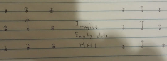
This is two separate localized field configurations- we might interpret this as two particles. But should we really have to adjust the phase angle of the all the fields over by the right particle if we are doing experiments only on the left particle?

Maybe what we really want is a local symmetry. A symmetry where we can rotate the phase angle of a phasor at any point individually (and all of them differently, if we like).

To Be Continued

A Roundabout Approach to Quantum Mechanics

More classical physics of paths

Semi classical light

Semi-classical particles

Basic special relativity

More Special Relativity and Paths

Special relativity and free will

We are doing Taylor series in calculus and it's really boring. What would you add from physics?

Why field theory?

Field theory implications

Planck length/time

More Physics Answers

In the standard model, what are the fundamental "beables" (things that exist) and what are kinds of properties do they have (that is, not "how much mass do they have" but "they have mass")?

What's the straight dope on dark matter candidates?

From SUSY

From GUTs

From Axions

If your results are highly counterintuitive...

Locality, fields and the crown jewel of modern physics